Hello Excellers, welcome back to another Excel tip today. I will show you how to create a self-expanding chart. This tip is also a YouTube Video. Why not check it out in the link below. So, it is really easy to create a self-expanding chart in Excel. Is it?. YES!. Normally a chart is set up to only display what is currently on the datasheet. But, by a few tweaks and Excel magic, we can set up a chart differently. We can allow a chart to automatically accommodate new data as it is added.
So, in Excel 2007 we can use a new table feature if you need the workbook to be backward compatible with previous Excel 2003 versions you need to do a few more clicks to get the same result. Let’s look at Excel 2007 and Excel 2003 first.
Create A Self Expanding Chart.
To create your self expanding chart in Excel 2007 and Excel 2003 do the following
- Create your chart as usual ( you can use the sample data below)
- Select any cell in the range that contains data that is used by the chart
- Choose Insert- Tables Tables to convert the range to a table

Note, if you are using Excel 2003 in Step 3 above choose Data- List-Create List.
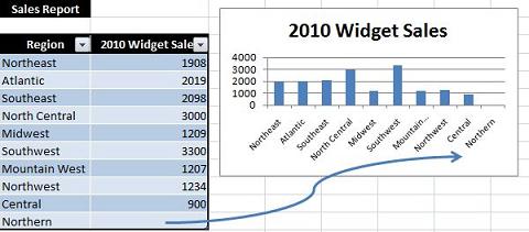
Believe it or not, that’s all there is to it!!. Excel recognises the data as a table and that any data that is added to it, is automatically updated in the chart.
So, as you can see in the screenshot above Northern has been added in automatically after I typed it then tabbed along to the Widget Sales ready for the figure to be entered. A great way to create a self-expanding chart in Excel.
Finally, give this charting technique a go, it a good one to have in your Excel magic box of tricks.