Hello, Excellers. Welcome back to another blog post in my Excel tips series. Today’s topic will show you how to re-order an Excel data series. When you create a chart in Excel, you may need to change how Excel displays your data series in your chart. For example, you may have a Minimum, Maximum and Average Sales price in your chart data.

The order in which you want to display the data may be Average, Maximum, then finally Minimum. You could change the order of the data in your data source in your worksheet range which would automatically change the order of the chart data display.
But, if you do not want to amend your source data, you can manually change the series order by customising the Excel chart.
So, let’s begin with some sample data.

I have already calculated my Minimum, Maximum and Average value sales for my products. Now, I need to create my Excel chart. Just follow the steps below.
- Select the data set
- Insert Tab
- Charts Group

- Click on the Insert Column Chart
- I want to insert a Column Chart
- By default, the Chart will be created with the default data series sequence specified in your data source

Change The Order Of Excel Data Series In 2013 Chart.
We want to change the data series sequence so the Average sales data in in the middle of our data seried, with Minimum on the left and Maximum on the right.
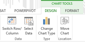
- Click on to the Chart to make it active
- The Chart Tools Options Tab will be visible
- In the Data Group Select – Select Data
- In the list of data series at the left of the dialog box, click once on the one you want to move.
- Use the Up Arrow and Down Arrow buttons to reposition the selected data series.
- When finished, click OK.
So, in this example I have moved the Average Data Series to the middle of the selection.

Change The Order Of Excel Data Series In 2016/365 Chart.
This blog post has now been updated for Excel 2016 onwards. Follow the steps below to re-order your Excel data series from 2016.
- Click on to the Chart to make it active
- Right Click in the Chart
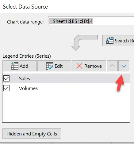
- Select Data
- In the select data source dialog box
- Use the up and down arrow in the Legend Entries (series) to change the Excel data series order.
- Hit ok
Want Even More Excel Tips?.
Finally, if you want to more Excel tips then feel free to bookmark my Macro Monday and Formula Friday blog post pages. They are updated every week.