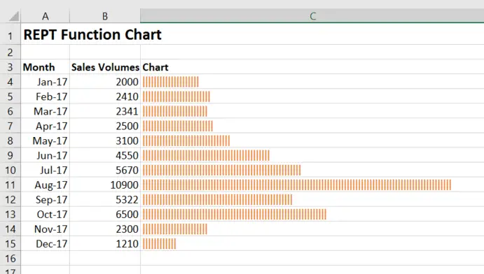
Hello Excellers it is Friday again and time for #formulafriday where we have some Excel formula fun. Have you used the REPT function in Excel or ever used it?. It’s a bit elusive so let’s get it out of the shadows and bring into the limelight as see how we can use it!. Are you ever short of space on your Excel worksheet? Did you know that you can create in-cell bar charts?. You can do so using the REPT function in Excel and produce a very handy Excel chart like the one below. They are really easy to set up and very simple to use.
Did You Know About The REPT Function?
In my experience, not that many people have heard of or use the REPT function. So what does it do?. The Microsoft Excel REPT function returns a repeated text value a specified number of times. The syntax of it is as follows-
=REPT(text, number_times)
With the following arguments.
text – this is a required argument, and is the text you wish to repeat.
number_times – this argument is also required and is a positive number specifying the number of times to repeat the text in the first argument.
Let’s get charting!. And Create An In Cell Excel Chart
So, follow the steps below to create your in cell Excel chart.
- Enter the REPT formula in the cell you want the chart to sit
- Use a divisor to make the length of the bars smaller
- Chnage the font to a more ‘chsrt like font’. I have used IMPACT
- Adjust the colour of the font to fit your overall theme
- Simple. An in cell chart with the REPT function in Excel
The formula I have used in this exmaple is
=REPT(“|”,B4/100) I have used 100 as the divisor to make the length of the cells more appropriate for the visual chart.
More Excel Charting And Formula Articles
If you want to follow all of my Excel articles for Formula Friday then bookmark my page. It is updated every Friday.
How To Excel At Excel – Formula Friday Blog Posts.