Happy Friday, Excellers, time for more #formulafriday #Excel fun. Today let’s look at how to split a cell that contains both text and numbers. When working with data in Excel, there are times when you need to separate the text from the numbers. For example, you may have a list of numbers you need to convert to text or vice versa. There are several ways to split text and numbers in Excel, and we will show you how to do it. Keep in mind that there is no one right way to do this, so feel free to experiment until you find the best method. Let’s get started!
I received data this week that had both a product description and product code in one cell. And I wanted to split the contents into two separate cells, one with the product description and one with the product code.

Solution 1. Use Text To Columns?.
The first solution I looked at was the Text To Columns feature. But, as the product description is different string lengths, I could not use the Fixed Width feature. However, if the data was uniform and all the product descriptions were equal in length, the Text To Columns would work.
Solution 2. Use A Formula. The MIN and FIND Functions.
So, it is time to turn to a Formula to help us out!!. It is a few formulas/functions, and it looks like this. First, we need to find the position of the first number in our cell. We do this using the following formula.
=MIN(FIND({0,1,2,3,4,5,6,7,8,9},B2&”0123456789″))

Now that we have the first number’s position (in positon 29), we can extract all numbers using the formula below.
=RIGHT(B2,LEN(B2)-MIN(FIND({0,1,2,3,4,5,6,7,8,9},B2&”0123456789″))-5)

This formula counts the number of characters that the first number Excel comes across. In our first cell, this is 29. We can use the RIGHT function to extract the characters after that position and return our numbers.
Note the -5 as we have the 500ml being five extra characters which we need to disregard from the calculation as Excel has correctly counted the first position of a number at 29 as it came across 5.
Have you used this method before?, Would you prefer to use the Flash Fill Method? Need to know what that is? Read on to find out.
Solution 3. Flash Fill (Excel 2013 onwards).
If you have aversion of Excel Excel 2013 or more recent then he Flash Fill feature can be used. Flash Fille which is noticeably quicker to acheive the same result but only in those versions of Excel where it is available.
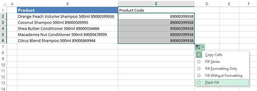
All you need to do is take the part of the data you want from the original cell, which is the Product Code paste or type into a new column, then drag the data down your cell until the Flash Fill icon appears, then hit flash fill.

When you release with cursor Excel will recognise the pattern of data in the data and fill the rest of the cells for you.

The Flash Full feature is definitely quicker than using formulas. However if you use earlier version of Excel the formula is a good solid option to work with. Which method do you use to split text and numbers in Excel?.

