Entering data into Microsoft Excel can be time-consuming for users. Especially if the cells that require data are spread all over the excel worksheet. The last thing you want is a user to the tabbing or clicking around the worksheet frantically looking for the correct cells to enter data. In particular if you need the user entering data in a specific order.
Excel CAN force the sequence of cells that you want users to select. So how does that work?. This solution relies on defining a named range which essentially is a sequence of cells that you specify. for more information on named ranges, I suggest reading my dedicated articles here
Formula Friday – 3 Reasons To Use Named Ranges In Your Excel Formulas
Write A Macro Which Highlights Named Ranges. Macro Monday.
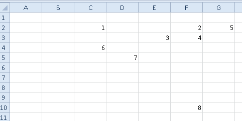
See below as an example of the sequence of cells that I want users to type into Excel. Pretty erratic isn’t it?.

So let’s give this a go.
Creating A Named Range
- Click in the cell that is second in your required sequence
- Hold down the CTRL key and click the cell sequence 3, carry on and select the cells in the correct order
- When you have reached your last cell in the sequence, click the first cell in the sequence
- Click the cursor into the Name Box (the area to the left of the bar that shows the cells addresses)
- Name this area of cells, i.e a named range in this example I am using MyDataSequence – then hit Enter and the name box will return to showing a normal cell reference
- Save your file
When you need to get a user to enter data into Excel in that order just select your named range MyDataSequence. Begin typing and press enter. Excel jumps to the next cell sequence ready for data entry
To view the details of the named range you created follow the steps below.
- Formula Tab
- Defined Names
- Name Manager
So, as you can see the named range is just a sequence of cells, that we selected earlier in the exercise. Give it a go.


