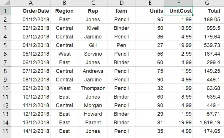
Hello Excellers, and welcome back to another #FormulaFriday #Excel tip in my Excel series. Todays article walks you through highlighting cells on an Excel worksheet that are locked. As an Excel user, you may have encountered a situation where some of your cells are locked. Users lock cells for various reasons, such as protecting formulas from being edited or preventing users from accidentally entering data into the cell.. One way to do this is by using the CELL function. This function will return a number that corresponds to the locked status of a cell. Let;s learn some Excel!.
So, if you have created a worksheet a long time ago and can’t remember which cells are locked, or if you inherit a worksheet and need to do the same, then this tip is very useful. Let’s go ahead and lock all of the UnitCost cells first.

Lock The Excel Cells.
Follow the steps below to lock your cells.
- Select the full worksheet by Ctrl +A+A.
- Home Tab | Cells Group | Format | Format Cells | Protection.
- Deselect or remove the tick from the locked option.
- Select the cells you want to lock on your Excel worksheet.
- Repeat the process above by selecting the tick option.
- Review Tab | Protect Group | Protect Sheet
With locked cells set, use conditional formatting in conjunction with the CELL function. The CELL function returns information about a cell.
The Syntax Of The CELL Function.
Here is a quick recap of the CELL Function syntax.
=CELL(info_type, [reference])
The CELL function syntax has the following arguments:
Info_type This is a required argument. A text value that specifies what type of cell information you want to return.
The following list shows the possible values of the Info_type argument and the corresponding results.

Reference This is an optional argument relating to the cell that you want information about. If omitted, the information specified in the Info_type argument is returned for the last cell that was changed. If the reference argument is a range of cells, the CELL function returns the information for only the upper-left cell of the range.
The Protect Info type is required. Excel returns the value 0 when the cell is not locked; otherwise, it returns 1 if the cell is locked. So, this information can be used with conditional formatting to identify locked cellsin the Excel worksheet.
Set The Conditional Formatting To Highlight Locked Cells.
- First, select the range to be formatted.
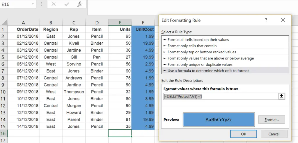
- Next, select Home Tab | Conditional Formatting | New Rule | Use A Formula To Determine Which Cells To Format. Enter the following formula.
=CELL(“Protect”,A1)=1
- Select the type of formatting to be applied if the result of the formula is true. Blue is selected in this example.

That’s it. Easy as that. In this blog post, we identified locked cells in Excel with the CELL Formula and conditional formatting. Locked cells appear highlighted with the formation chosen by the user. What an easy way to highlight locked cells. Do you have an alternative?. Please share in the comments below so other Excellers can learn.
I hope you found this information helpful! If you’re looking for more help with Excel, be sure to check out our other posts or contact us for assistance. Don’t forgot to check out my You Tube Channel for more Excel skills.
Finnally, for more Excel and VBA tips then sign up to my monthly Newsletter where I share 3 Excel Tips every month. You will receive my free Ebook, 50 Excel Tips.
Likewise, if you want to see all of the blog posts in the Formula Friday Series Click The Link Below
How To Excel At Excel – Formula Friday Blog Posts.
So, Don’t forget to SUBSCRIBE to the How To Excel At Excel Newsletter for more monthly Excel tip. Simply click on the link and enter your email. No spam. Just Excel tips.

