Hi Excellers, this is a different #formulafriday in my Excel 2020 series.  I want to share with you 3 ways to protect your Excel formulas.

So, you have spent a long time preparing your Excel spreadsheet solution, and I bet you don’t want anyone to mess up it up.  So there are a few ways to protect some of those most vulnerable parts of your Excel spreadsheet.

Here are my top 3 ways to protect your Excel Formulas!!

1. Hide them
2. Lock Cells
3. Hide The Formula Bar With Some Simple VBA.
4.  

1.Hide The Formulas.

This method will temporarily hide your formulas, but you will be able to use them again if you need to.  It’s simple and straightforward.  Here we go.

• Select all of the cells that contain formulas that you want to hide.
• Home Tab – Cells Group – Format – Format Cells
• Navigate to the Protection Tab
• Check the Hidden option and hit Ok

This doesn’t in itself hide your formulas, you need to then protect your worksheet to ensure these settings work.

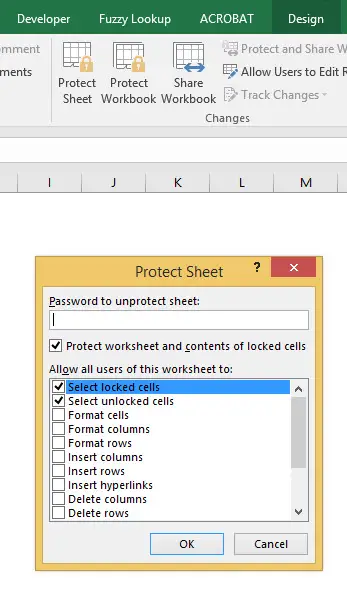
• Select Review Tab
• Changes Group
• Select Protect Sheet
• Enter a password and confirm password when prompted
• That’s all you need to do.

Try selecting a cell that contains a formula.  The formula will not be visible in the formula bar.  If you want to see the formulas again simply unprotect your worksheet.

2. Lock Cells.

The second method is to just lock the cells that contain formulas so they cannot be selected or edited by users. By default all cells in a workbook are locked, so you will need to unlock them all to start with.

• Hit CTRL+A to select all of the cells on the worksheet
• Home Tab – Cells Group -Format – Format Cells
• Untick Locked, to unlock all of the cells on the worksheet
• Hit Ok

Now all we need to do find all of the cells that contain formulas..

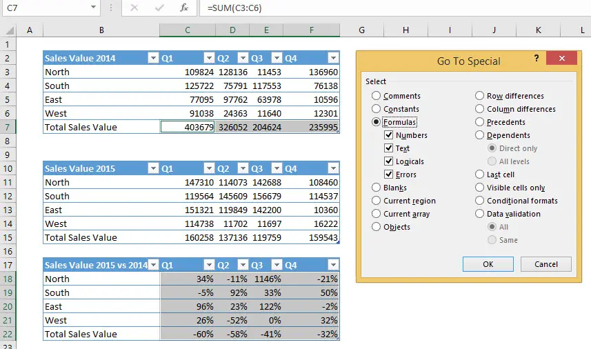
• Hit F5 to bring up the GoTo Dialog Box
• Select Special – Formulas – Hit OK
• All of the cells that contain formulas will be highlighted

Then we need to lock those highlighted cells.

• Home Tab – Cells Group -Format – Format Cells
• Navigate to the Protection Tab
• Check the Locked option and hit Ok

This doesn’t in itself lock your formulas, you need to then protect your worksheet to ensure these settings work.

• Select Review Tab
• Changes Group
• Select Protect Sheet
• Enter a password and confirm password when prompted
• That’s all you need to do.

3. Hide The Formula Bar With Some Simple VBA

My third method of hiding your formulas is to actually hide the formula bar on the Excel worksheet.  This is easily achieved by a very small piece of VBA coding or an Excel Macro.

This macro uses the Application Object and we are looking to use the DisplayFormulaBar property of it.

To use this small piece of coding, you need to insert it into a module in your Excel workbook.

•  Open Visual Basic – by hitting F11 or Developer Tab – Visual Basic – Click Modules, and Add New Module.

Here is the VBA code if you want to copy it.  Just paste it into a module you have created as per the instructions above.

Sub HideFormulaBar()
    Application.DisplayFormulaBar = False

End Sub

Just as we have hidden the formul bar we can easily write some VBA to show the formula bar again

Sub ShowFormulaBar()
    Application.DisplayFormulaBar = True

End Sub

In this instance we set the Application.DisplayFormulaBar to TRUE to display the formula bar.

That’s it. Hope you enjoyed Formula Friday.

Don’t forget to sign up to the Excel at Excel Newsletter for 3 free Excel tips monthly. Just click on the Sign Up Form to the right or use the link below.