Hello, Excellers. Welcome to another instalment of #formulafriday. Today let’s look at here a handy Excel Tip if you want to highlight today’s date in your Excel data set. I have found this really useful visually where I have sequential dates and want to see where today’s date sits in the sequence. You can see from my example data set below, I can easily see today’s data with some simple conditional formatting. (..and let’s say today’s date is 28/12/2017).

There are a few ways to always highlight today’s date, but let’s look at two of them.
Use Conditional Formatting To Highlight Today’s Date
This is a handy way to use the conditional formatting function.
- Highlight the column of data that contains your incremental dates data
- Home Tab | Styles Group | Conditional Formatting
- Select New Rule | Use a formula to determine which cells to format
- In the Formula Dialog box type, the following formula which compares the date in Column A to today’s date and if it matches then the cells are formatted as you have specified. The $ in front of A in the formula always looks at Column A irrespective of the location of the cell you are highlighting
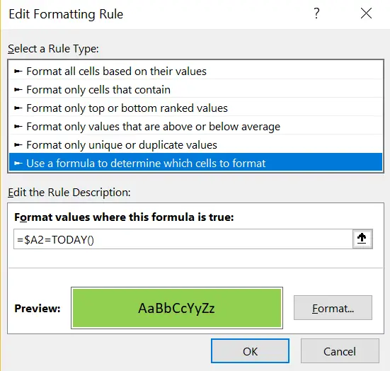
- Just choose a type of formatting then hit Ok. I have chosen to highlight the cell GREEN if the date matches today’s date.
Use A WINGDINGS Symbol To Highlight Today’s Date.
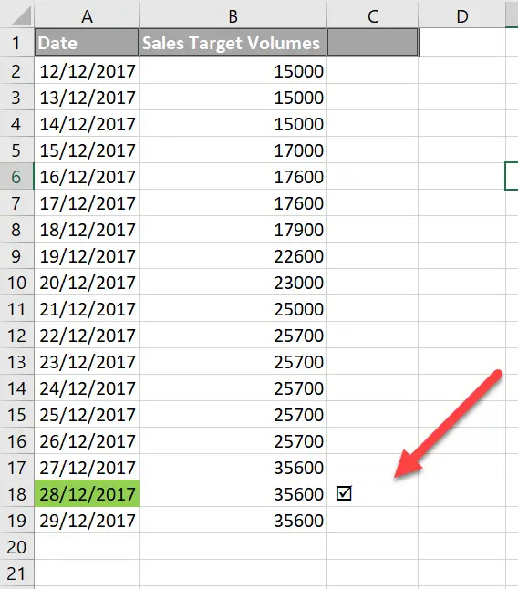
This second method takes a little more setting up but adds a little more visual conditional formatting to your Excel worksheet. You will end up with something that looks like this below. Either across (above) your row of dates, or down the side of your column of date. I have chosen in this example to use an arrow to point to today’s date within the date sequence in Column C.
It is similar to the first method as it uses conditional formatting to draw attention to today’s date. This method of conditional formatting little more imaginative using a symbol from the WINGDINGS font.
- Highlight cell C2 | Insert |Symbol
- Under the Font Tab Select WINGDINGS | Select your Symbol
- Double click to fill the series of data down your column
- You should now see a series of the symbol that you have selected down your whole column of data
- The last step is to change the font to white (or the same background as your worksheet) this makes the symbols ‘disappear’, or gives the illusion that they have disappeared.
All we now need to do is repeat the process of conditional formatting with the same formula as above
- So, we still want to look at the date in Column A to see if it is equal to today’s date, but this time we want to format Column C.
- Click Format | Format Cells | Font and select the colour of the font. In my case, I have selected Automatic which is Black for the conditional formatting.
Wrapping Up.
That’s all we have to do. Whenever you open the workbook, the current days’ date will be highlighted in whatever way you have chosen. You could get quite artistic!. Do you think it’s a cool way to highlight dates?. Let me know in the comments below if you have used this method of conditional formatting.
So, What Next? Want More Tips?
If you want more Excel and VBA tips then sign up for my Monthly Newsletter where I share 3 Tips every month and receive my free Ebook, 50 Excel Tips and check out all of my Formula Friday Blog posts below.
How To Excel At Excel – Formula Friday Blog Posts.