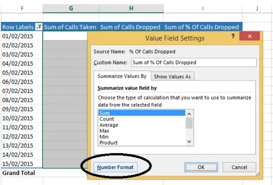
I have seen this a lot with Pivot tables, the frustration of Excel users when they format their data in a Pivot Table, but they hit refresh or they remove and add back data into the calculations area and boom the formatting has gone. Take a look at my data extract of call centre numbers.
I have the data of calls taken and calls dropped for a period of time in February 2015.
I have added in a calculated field to my Pivot Table (if you want to read more about that you can check out my blog post right here). My calculated field is the number of calls dropped as a percentage of the total number of calls taken that day. A pretty standard calculation.
I have gone ahead as users sometimes automatically do and highlighted the cells direclty where the calculation in and change it to %. ( ohh seems like this maybe where we are going wrong??????)….
This changes my calculated field to a %, but if I then remove the value fields then decide to add in the Sum of Calls Dropped field. See what happens. Yes that right the formatting sticks to the cells rather than the data values.
Easily resolved.
- In Excel 2013- Clikc on the Pivot table to enable the PivotTable Fields view
- In Values select the data set you want to format- in this case it is the % of Calls Dropped
- In Value Field Settings, select Percentage
- Hit Ok
Your number formatting now only relates to that value field. By setting a number format on the field itself, the number format will be applied consistently no matter how much the table changes. Phew that another Excel annoying problem solved.
Want more Excel Tips?. My Free Newsletter every 15 days has 3x Excel tips. Just click Here To Sign Up or Fill in the box on the right.
Create Multiple Reports From One Pivot Table
Break Your Pivot Table Filters Into Multiple Columns


