Hello, Excellers. Time for some more #Macro fun. If you’ve ever needed to convert a range of cells in Excel to lowercase, you’re in luck!. In this post, I show you how to create a macro that will automatically change the case of cells to lowercase. I also provide instructions on how to use the macro. So, whether you’re just getting started with macros or are an experienced user, this post is for you! Happy coding!
So, you may (or may not) know that you can change the case of text to a lower case using the Excel LOWER function Excel. Alternatively, a small bit of Excel VBA code will do the same over and over again automatically. Let’s get writing some simple VBA.
What Does The Macro Do?
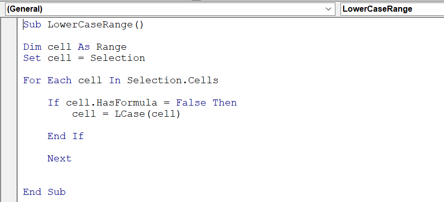
This macro converts any range of cells that the user selects into LOWERCASE, only if the cells contain a string.
Prepare To Write The Macro.
First, open the Visual Basic Editor. There are two ways to do this.
- Hit ALT +F11 or
- Select the Developer Tab | Code Group | Visual Basic. Both methods have the same result.
So, if you cannot see the Developer Tab you may need to enable it. Check out my very short YouTube video for instructions. Learn how to enable the developer tab in just a few minutes.
Where To Store The Excel Macro?.
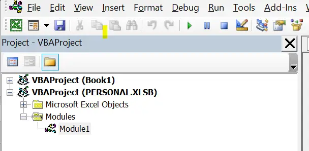
Next, where to save your Excel macro?. So, you can either save the code in your current workbook or in your Personal Macro Workbook. If you want to reuse the macro over and over again (like this one) in many workbooks save it in the Personal Macro Workbook. To use the code only in the current workbook, save it in the current workbook. In this case, it makes sense to be able to access this macro for any workbook. Therefore, the code is stored in my Personal Macro Workbook.
Step 1. Insert A New Module.
The first step is to insert a new module into the workbook (either the current workbook or as stated already this one goes into my Personal Macro Workbook).
Hit the Insert Menu | Module. So, once the new module is inserted, type Sub then the name of the Excel macro. In this example, I have named my Macro LowerCaseRange. The End Sub ending code is inserted once a new macro is created. Any other lines of code are placed in between these two lines of code.
Sub LowerCaseRange()
End Sub
Step 2. Declare Any Variables.
One variable needs to be declared. This allocates a memory container for the range of cells selected by the user to convert to lowercase.
Dim cell as Range
Step 3. Set The Range To Convert To Upper Case.
Next this the code below sets the range that the use has selected as the range of cells to convert to lowercase.
Set range = Selection
Step 4. Check For Cells That Contain Formula. Convert Cells If They Do Not.
The For Each looping method checks if any of the cells in the selection contain a formula. This is ideal. It executes a statement or a group of statements for each element in an array or collection. If any cells contain a formula then they are not converted. If they are not or ‘False’ then Excel goes ahead and converts the cells to lower case. This continues until all of the cells in the selections have been looped.
For Each cell In Selection.Cells
    If cell.HasFormula = False Then
        cell = LCase(cell)
    End If
    Next
Step 5. Ending The Macro.
So, once all of the cells in the selected range have been converted to lower case then the code ends. This bit of code was automatically generated as the macro was named in the first stage of writing the code. Nice.
Then my favorite step test your code!
Want To Copy The Code?
Sub LowerCaseRange()
'macro by HowToExcelAtExcel.com
Dim cell As Range
Set cell = Selection

For Each cell In Selection.Cells

    If cell.HasFormula = False Then
        cell = LCase(cell)

    End If

    Next


End Sub
In addition, if you want to see all of my blog posts in the Macro Mondays Series you can find them all in the link below. Why not bookmark it? New Conect Every Monday.
How To Excel At Excel – Macro Mondays Blog Posts.
Note. Always make a backup copy of your work before running any macros.

