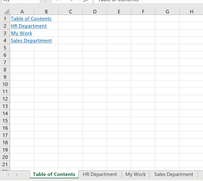
Hello, Excellers. Welcome back to another #MacroMonday #Excel blog post in my 2021 Excel series. I love this macro. I really do. It is great to have it to hand when needed. This small bit of code will automate the creation of a table of contents in your Excel workbook. Yes, that is right. In short, run this code and Excel inserts a new worksheet with links to all of the sheet tabs with a hyperlink automatically. So, that is a good bit of time-saving right?.

Prepare To Write The Macro.

First, open the Visual Basic Editor.  There are two ways to do this. 

• Hit ALT +F11 or
• Select the Developer Tab | Code Group | Visual Basic.  Both methods have the same result.   

So, if you cannot see the Developer Tab you may need to enable it. Check out my very short YouTube video for instructions. I will show you how to enable the developer tab in just a few minutes.

Next, you need to decide where to save your Excel macro. So, you can either save the code in your current workbook or in your Personal Macro Workbook. If you want to reuse the macro over and over again in many workbooks save it in the Personal Macro Workbook. If the code is only to be used in the current workbook, save it there. As this a macro that could be used over and over again to created content tables in many workbooks I will save it in my Personal Macro Workbook.

Here Is The Code.

Sub TableofContents()

Dim i As Long
On Error Resume Next

   Application.DisplayAlerts = False
     Worksheets("Table of Contents").Delete
    Application.DisplayAlerts = True

On Error GoTo 0
ThisWorkbook.Sheets.Add Before:=ThisWorkbook.Worksheets(1)
ActiveSheet.Name = "Table of Contents"
For i = 1 To Sheets.Count
With ActiveSheet
.Hyperlinks.Add _
Anchor:=ActiveSheet.Cells(i, 1), _
Address:="", _
SubAddress:="'" & Sheets(i).Name & "'!A1", _
ScreenTip:=Sheets(i).Name, _
TextToDisplay:=Sheets(i).Name
End With
Next i
End Sub

Step 1. Insert A New Module

The first step is to insert a new module into the workbook. Just hit the Insert Menu | Module.

So, once the new module is inserted, type Sub then the name of the Excel macro. In this example, I have named my Macro TableOfContents(). Excel automatically inserts the End Sub ending code once a new macro is created. Any other lines of code are placed in between these two lines of code.

Sub TableofContents()
End Sub

Step 2. Declare Variables.

Moving on. the next step is to declare any variables. This creates a memory container in Excel for any values we want Excel to store. In this macro one variable need to be declared.

Dim i As Long

Step 3.

So, in this next step, we take into account errors that might happen. By the line of code below, we can choose to ignore any errors and let the macro continue to run. This is absolutely fine for this part of our macro, but on other macros, you may not want to let the code carry on. So, my advice would be to use caution.

I have chosen to use this to allow Excel to move on from any errors that occur when running lines of code in steps 4 through 6. (Deleting any current table of contents pages). This line of code goes to the statement immediately following the statement where the error occurred, and execution continues from that point.

On Error Resume Next

Step 4. Turn Off Any Screen Alerts

Next, any screen alerts that may have popped up on the screen are turned off. This prevents the user from having to deal with any unnecessary messages from Excel.

Application.DisplayAlerts = False

Step 5. Delete Worksheets Already Named Table Of Contents.

This next bit of code deletes any worksheets already named Table Of Contents. This a small but handy step. Once the macro is run over and over again, to add new worksheets to the table of contents there is no conflict.

Worksheets("Table of Contents").Delete

Step 6. Turn Display Alerts Back On

It is with this line of code that Step 4 is reversed. As a result, display alerts are turned back on.

Application.DisplayAlerts = True

Step 7. Handling Errors In Creating The Table Of Contents.

This next line of code allows Excel to go to the statement immediately following the statement where the error occurred. Execution continues from that point.

On Error Goto 0

Step 8. Add A New Worksheet Names Table Of Contents.

Next, a new Worksheet is added at the beginning of the worksheet (before worksheet 1). This is named as Table Of Contents.

ThisWorkbook.Sheets.Add Before:=ThisWorkbook.Worksheets(1)
ActiveSheet.Name = "Table of Contents"

Step 9. Enumerate All Worksheets In Table Of Contents.

Here, i begins the count of how many worksheets are in the workbook. The counter begins at 1 and ends at the maximum count of all sheets in the workbook. Finally, when the maximum number is reached, the macro ends.

For i = 1 To Sheets.Count

Step 10. Add The Hyperlinks for The Table Of Contents.

Next, use the Hyperlinks.Add method to add the sheet name and hyperlinks to the cell. This step feeds the Hyperlinks.Add method the parameters it needs to build out the hyperlinks

With ActiveSheet
.Hyperlinks.Add _
Anchor:=ActiveSheet.Cells(i, 1), _
Address:="", _
SubAddress:="'" & Sheets(i).Name & "'!A1", _
ScreenTip:=Sheets(i).Name, _
TextToDisplay:=Sheets(i).Name
End With

Step 11. Looping Back

This step loops back to the increment the count of i to the next count. Once all of the worksheets have been counted the macro finally ends in step 12 below.

Next i

Step 12. Ending The Macro.

Finally, the macro ends once all of the worksheets have been looped through and the hyperlinks added. This line of code has already been added when the name of the macro was entered way back in Step 1.

End Sub

That is it. This macro can be re used over and over again if stored in your Personal Macro Workbook. Time to test it!.