In this blog post, I will show you how to easily remove multiple hyperlinks from an Excel workbook. I recently had this question submitted via email from a subscriber. They had a LOT of hyperlinks in an Excel workbook (with 50+ sheets), and they wanted to quickly remove all of the hyperlinks as they were no longer relevant.  It is easy to remove multiple hyperlinks from a single worksheet, but removing hyperlinks from multiple worksheet tabs requires a little more work.  Let’s work through them both, starting with removing hyperlinks from a single Excel worksheet.

Remove Hyperlinks From A Single Excel Worksheet.

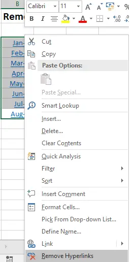
• Select your range of cells that contain the hyperlinks
• Right Click | Remove Hyperlinks

That is simple right. All hyperlinks are now removed from the single Excel worksheet

Remove Hyperlinks From Multiple Worksheets.

You would expect maybe to be able to simply group all of your worksheets and then repeat the actions above on multiple worksheets, this is not the case, unfortunately.  You can either repeat the above procedure for all of your worksheet tabs, but if you have over 50 then it would become a chore,  instead, we can write a tiny bit of Excel VBA code, (a Macro) to remove the hyperlinks all at once with the click of a mouse.  Sound good?. Then here how simple it is.

• Hold down the ALT + F11 keys to open the Microsoft Visual Basic for Applications window.
• Click Insert > Module, and paste the following code in the Module Window.

Sub RemoveAllHyperlinks()
Dim ws As Worksheet
For Each ws In ThisWorkbook.Worksheets
ws.UsedRange.Hyperlinks.Delete
Next ws
End Sub

• Press F5 key to run this code. Excel removed all the hyperlinks from the active worksheet immediately.

Let’s Walk Through The Code.

Step1. Start The Macro.

First, insert a new module. This can be in the current workbook or in your Personal Macro Workbook. What is the difference?. To reuse the code over and over again, save the code in a module in your Personal Macro Workbook. If you want to read more about the Personal Macro Workbook then feel free to read my blog posts below.

• Macro Mondays – How To Remove All Hyperlinks From An Excel Workbook
• Macro Mondays – How To Write A Macro To Delete All Hyperlinks In Your Excel Workbook
• Make Your Excel HyperLinks Dynamic – Formula Friday
• Make Your Excel Hyperlinks Dynamic – Using The Hyperlink Function – Formula Friday
• Excel Tip- Formula Friday -How To Create a drop down list for your hyperlinks in Excel

Type Sub and then the name of your macro. In this example the macro is named RemoveHyperlinks. Once this first line of code is entered, the End Sub line of code is entered automatically. All other lines of the macro code are typed in between these two lines.

Step 2. Declaring Variables.

Next, any variables need to be declared. This allocates memory in Excel to store these values. There is only one variable in this macro.

Dim ws As Worksheet

Step 3. Looping Through All Worksheets.

The next part of the code is using the For Each Lopping method. The code loops through a used range of cells in the first worksheet in the active workbook. Excel deletes any hyperlinks. Once all hyperlinks have been deleted the next worksheet is looped. This continues until all of the worksheets in the workbook have had hyperlinks deleted.

For Each ws In ThisWorkbook.Worksheets
ws.UsedRange.Hyperlinks.Delete
Next ws

Step 4. Ending The Macro.

So, once all of the the worksheets in the workbook have been looped and the hyerlinks deleted the macro ends. This line of code already exists and Excel inserted this at the time the macro was named.

End Sub

If you want more Excel and VBA tips then sign up to my monthly Newsletter where I share 3 Excel Tips every month and receive my free Ebook, 50 Excel Tips.

If you want to see all of the blog posts in the Macro Mondays Series or the example worksheets you can do so by clicking on the links below.

How To Excel At Excel – Macro Mondays Blog Posts.