I like to cut down on actions that constantly require you to manualy repeat them. I like to do things once, then just re-use the process of possible. That is why this is such a great time saving tip. Let’s see how to create a customised view of our Excel worksheet that we can choose from a list, that is tailored to our own preferences that we have saved right there in the Excel workbook. Customised Views….let’s go.
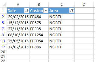
So here is a workbook that I use, often, and I like to look at the most recent entries at the top of the screen, filtered to the Northern Area. This is my go to view even though there are entries in the workbook for East, West and South Regions.

It is SO easy to create a custom view. Customised view can contain settings for the following features-
column widths, row heights, hidden rows and columns, cell selections, filter settings, and window settings, and print settings -page settings, margins, headers and footers, and sheet settings.
Do all of the formatting, filtering and print settings you want to to be your go to view.
- View Tab
- Workbook View
- Custom Views
- Add View
- Name your view- I have named mine my NORTHERN view


No matter what view the workbook is left in, another user may have left all of the data showing, but that’s ok, we can quickly get our go view.
- Hit Custom View
- Select your names view and hit Show
- You own personalised view appears!
Want To Watch The Video?

- Hide all of your Excel formulas from prying eyes!
- Undertand and debug Excel formula errors
- How To Display a Plus + Sign On Positive Numbers With Custom Formatting In Excel
- Create A Timestamp In Excel With Formulas

