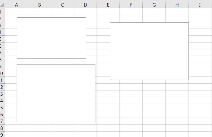
Hello Excellers, it is time for another #macromonday blog post. Today let’s look at one handy little macro that will re size all charts on your Excel worksheet with the click of a mouse, or the runing of s simple bit of VBA code. I know that sometimes when I create charts on an Excel worksheet they are not always the same size and to resize can take up a lot of time. Even selecting them to change as a group takes time. Therefore, this code will take a worksheet full of charts like the ones below and automatically re-size them to whatever size you specify.
What Does The Macro Do?.
It loops through all of the charts in your Excel worksheet and changes the width and height to the size that you specify within the code.
How Does The Macro Work?.
The macro uses the For Next looping function which is one of the most powerful VBA procedures which allows you to loop through code a fixed number of times. This, therefore sounds an ideal process for us and we want to loop every chart and change the size of it. The syntax of this procedure is really simple.
The syntax to create a FOR Loop using the FOR…NEXT statement in Microsoft Excel is
For counter = start To end [Step increment] {…statements…}
Next [counter]
Stepping Through The Code.
Step 1. Activate the Visual Basic Editor By hitting ALT+F11 shortcut of you can go to the Developer Tab | Visual Basic to open the Visual Basic Explorer Window. If you want to know how to enable the developer tab then you can check out my YouTube Video below for some simple Instructions.
Step 2. We need to declare a variable. In this case it is our counter which we delare and an Integer. This enures that a memory container is allocated for this value.
Dim I As Integer
Step 3. Excel begins to loop through all of the charts in Excel worksheet one by one using the looping process and using the With…End Wtih we can execute Step 4 without contiually refering to to the ActiveSheet.Object.
Step 4. The Width and Height of the charts is specified at this stage. Therefore, in this example I have chosen to set the chart size as 500 by 400, but this is where you can change the code to suit your requirements.
Step 5. FInay, once all of the eight and width of the charts have been updated to 500 by 400 then the loopings ends.
Step 6. The routine ends with the End Sub coding.
Step 7. Finally, you can test your Macro. (Of course my favourite step!)
So, that’s it folks. I find this really useful if I have a lot of charts or mini charts in particular that can be frustrating a fiddly to change. I hope you find this piece of code useful. Let me know in the comments below if you have used it.
Want To Download The VBA Code?
Sub ResizeCharts()
‘Macro by How To Excel At Excel
Dim I As Integer
For I = 1 To ActiveSheet.ChartObjects.Count
With ActiveSheet.ChartObjects(I)
.Wdith = 500
.Height = 400
End With
Next I
End Sub
What Next? Want More Excel Tips?
So, if you want more Excel and VBA tips then sign up for my Monthly Newsletter where I share 3 Tips on the first Wednesday of the month and receive my free Ebook, 30 Excel Tips.

If you want to see all of the blog posts in the Macro Monday series. Click on the link below
How To Excel At Excel – Macro Mondays Blog Posts.
Do You Need Help With An Excel Problem?.
I am pleased to announce I have teamed up with Excel Rescue, where you can get help with Excel FAST.


 </a
</a