Hello Excellers and welcome back to another #Excel #FormulaFriday blog post in my 2020 series. Today I will show you to use a dynamic column reference with the VLOOKUP formula.
Working with large data sets you may need your VLOOKUP to dynamically update the COLUMN argument as you copy or drag your formula across. If you do then you need to know how to use VLOOKUP with the COLUMN function.
Step Back. The VLOOKUP Formula Syntax.
Let’s take a reminder of the syntax of the VLOOKUP formula.
=VLOOKUP(lookup_value,table_array,col_index_num,[range_lookup])
Where
- Match = What you want Excel to find
- Table Array = Where you want Excel to look for it
- Column Number = If Excel finds it, how many columns from the left is the data you want?
- Range Lookup = Optional hence in the brackets, False= Exact Match, True= Approximate Match
So, when we specify FALSE as the Range Lookup where we want an EXACT match Excel goes through every single record, it can be slow, it is carrying out a linear search.
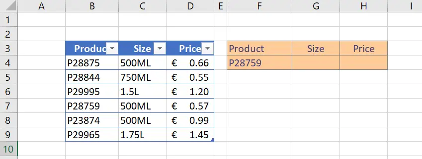
Always better to work with an example, so that is what we will do. My data set is below. (This is a small extract my data set has thousands of lines). It is a simple list of Products along with Size and Pricing. You can also see that I want to use a VLOOKUP to find the Size and Price of particular product in my data return area in cells F3 to H3.

As you can see I would need the col_index_num argument of the VLOOKUP function to dynamically move as I drag the formula across. I would normally have to write two formulas like below to retrieve the information.

Instead of hard coding the columns numbers into the VLOOKUP we can use the COLUMN function. COLUMN translates a column number into a cell address. This saves a LOT of time instead of writing TWO VLOOKUPs!
So if we type Column(A1) then the result is 1, then type B2, the result is 2 and so on. Ah, this may be useful right?.
The Dynamic Formula.
The first COLUMN INDEX NUMBER in the VLOOKUP I want to return is in the SECOND column of our data set, so instead of using 2 as the COLUMN INDEX NUMBER, I can replace it with B1. The formula looks like this.
=VLOOKUP($F$4,Table1,COLUMN(B1),FALSE)
I can now drag the formula across and return the next column automatically. How COOL is that right?. Using a Dynamic Column Reference With VLOOKUP. Job Done.
