Hello Excellers, welcome to another #Excel #FormulaFriday blog post in my Excel series. Today let’s explore the UNIQUE function in Excel. This newly released function is part of the DYNAMIC Array functions announced by Microsoft back in 2018. At that time these array functions were only beta release available to a portion of Office insiders. A few days ago, Microsoft announced these awesome new Excel functions are now available to the Excel monthly Channel. So without any delay let’s get down to using the UNIQUE function.
What Does The Unique Function Do?
This new function in Excel will return a list of unique values or a list of values that occur only once from an array. What is an Array?. In Excel, this is just a list of items or a structure that holds a collection of values. These values can be text, dates, numbers etc. 
The Unique Function Syntax.
First, let’s go over the arguments that construct the UNIQUE function. =UNIQUE(Array,[By_Col],[Exactly_Once]) Where Array – This is the range or array from which you want to return unique row or columns. By_Col – this is an optional argument, as it has the [] brackets. This is a logical value, compare rows against each other and return unique rows = FALSE or is omitted; compare columns against each other and return the unique columns = TRUE. Exactly_Once – this is also a logical value and another optional argument. Returns rows or columns that occur exactly once from the array = TRUE; to return all distinct rows or columns from the array = FALSE or omit
Extracting Unique Values From ROW Array.
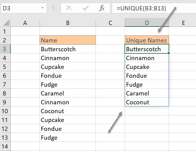
For example, take a look at my list of items below
It is easy with the Excel Unique Function to now return a list of Unique names from this list. The formula =UNIQUE(B3:B13) . As illustrated below.

Excel will ‘spill’ the unique names and create a new array for you.
Extracting Unique Values From COLUMN Array.
Do note, however, that by not using the optional argument of By_Col, the argument has defaulted to FALSE which will return unique ROWS. If my array was in columns then I would simply adjust the formula to set the By_Col to TRUE. I have adjusted the array to COLUMNS.  So, as you can see it is really easy to extract our UNIQUE values. There is one other argument which is also optional which can give us another flavor of the Function. It is the Exactly_Once argument. What is that?. Well, this option will determine how the function deals with repeating values. By leaving the default to FALSE, Excel will extract unique values regardless of how many times they appear in the array or source of data. If we set this optional argument to FALSE then this now changes things a LOT. The UNIQUE function will extract ONLY VALUES THAT APPEAR ONCE.
Extracting Values That Appear Only Once.
Finally, let’s test this out with our data set. Moving back to my example column of data. If we want to return only those values that appear once then the formula is
=UNIQUE(B3:B13,FALSE,TRUE)

How easy is that?. An Excel array function that is now available to most Excel users. It is part of a new release of array functions.
What Next? Want More Tips?
So, if you want more tips then sign up for my Monthly Newsletter where I share three Excel tips every month and receive my free Ebook, 50 Excel Tips.
Do You Need Help With An Excel Problem?.
Finally, I am pleased to announce I have teamed up with Excel Rescue, where you can get help FAST. All you need to do is choose the Excel task that most closely describes what you need to be done. Above all, there is a money-back guarantee and similarly Security and Non-Disclosure Agreements. Try It!. Need Help With An Excel VBA Macro?. Of course, you don’t need to ask how to list all files in a directory as it is right here for free.


