Welcome to Session 4 of Pivot Table Week.

Thanks for joining me again for Session 4 in Pivot Table Week.  Today we will be looking at additional calculations in

 

If you need a recap of previous sessions you can view them below

 

 

Session 1 What Are Pivot Tables

Session 2 Create Your First Pivot Table

Session 3 Pumping Data With The Pivot

 

Pivot Table Calculations.

By default Excel will populate the Value area of your Pivot Table by appliying the SUM function to any numeric field you put there or indeed will apply the COUNT function to any non numeric field.

You can however choose from a large selection of calculations as well as adding our own custom calculated fields to the table.  To use a different summary function or calculation just right click any cells in the values area of the Pivot Table, then hit Value Field Settings.  Excel will display the Value Field Settings dialog box, just selection the function  you want from the Summarise Value By List.

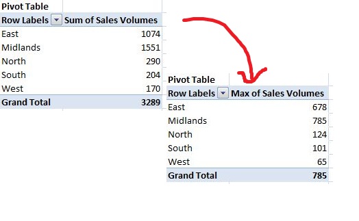
In the example below, I have changed the SUM of Sales Volumes to the MAX of Sales Volumes, you will see the Custom Name chnages also from SUM to MAX.

 

Using Custom Calculations

In addition to the standard summary function explained above Excel also can provide you with some custom calculations and with these you can have each item in your Values area of the Pivot Table.  With these custom calculations you can have each item in the Values area of your Pivot Table as a % of the total values in the same rows or columns, create running totals, or show each value as a % of of some base value.

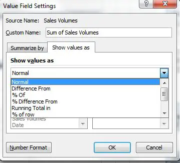
If you want to  apply one of these customer calculations then just right click a cell in the Values area, then click the Show Values As List.  Then just select from the options available- see them below.

 

 

 

 

 

 

 

 

 

 

 

 

In my example I have chosen to show the Sales Volumes Per Area not as totals but as a % of the Total Sales, with just a few clicks.

 

If this is STILL  not enough calculations for your needs the Excel let’s you Create …..

 

Calculated Fields and Items- some facts

• A calculated field an addtional new field that is derived from calculations you base on existing fields in your Pivot Table.
• A calculated item is is a new item that you create in an existing field derived from calculations performed on other items that are already in the field.
• Once created Excel makes the fields and items available as thought it were part of your data source.
• Custom field and items can apply arithmetic operations to any data already in your Pivot, but cannot reference outside your Pivot Table. 

Now we have the facts out of the way let’s get CALCULATING A FIELD

 

To create a calculated field

• Select any cell in the Pivot Table.
• Under Pivot Table select  Tools then hit Formulas
• Select calculated field
• Insert calculated field dialog box will appear
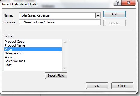
• Type a name for your calculated field in the Name Box
• Type your calculation

In the example below lets calculate the Total Sales Revenue

Which gives us the resultant Calcuated Field Total Sales Revenue

We can now work with the new field using the same techniques you use to work with existing field in your Pivot Table.

 

Let’s get CALCULATING AN ITEM

When creating a calculated item for a field just select any existing item in the field or the field headings. 

• Under Pivot Table Tools
• Click Options Tab
• Pivot Table Tools
• Formulas
• Tools Group
• Calculated Item

In my example below I have chosen to calcuate a new item of NorthEast Sales Volumes.

Note- you cannot create calculated item in field that have custom subtotals.

See you for Session 5. Grouping And Ungrouping Pivot Table Data.