Hello, Excellers welcome to another blog post in my 2019 #FormulaFriday #Excel tips series. Today let’s take a look at creating a formula or a calculation within an Excel Pivot Table.
If you want to go back to basics and learn the basics then you may want to view my YouTube Video on Creating Your First Pivot Table.
But, if you are happy enough with Pivot Tables and are keen to up your skills even more then read on to find out how to use Calculated Fields.
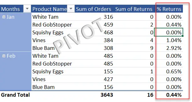
In this example, I want to calculate the percentage between two of my fields. In particular, the number of Sales Returns vs Sales Orders i.e what percentage of my Orders have been subsequently Returned. We will be working with my data set below.

What Are Calculated Fields?.
I like to think of a calculated field as a virtual extra column of data I have added created from other existing columns from the Pivot Table. For example in our data set up, we have the number of sales and the number of returns for each product. This means we do not have to write a formula, apply the formula to our data set or check that any new lines of data added have been updated also with this formula. Sounds like a good solution right?.
Adding A Calculated Field To A Pivot Table.
For example we want to calculate the % of returns of our sales orders. We have both of these fields in our Pivot Table.
- Select any cell in your Pivot Table
- Pivot Table Tools | Analyze
- Calculation Group | Fields, Items & Sets
- Select Calculated Field from the drop-down list

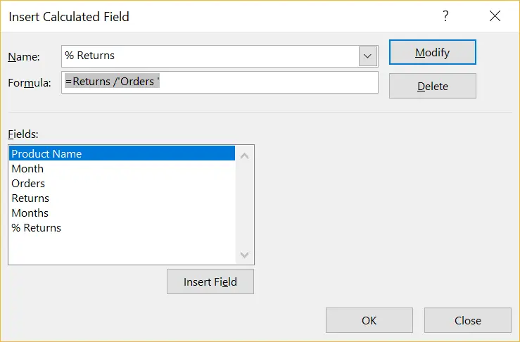
- Give your Calculated Field a name by filling in the Name part of the dialog box. I am calling this example % Returns.
- Go ahead and write your formula. Choose your fields from the field list below the formula box. You can manually type the formula or double click to use the fields you require. In my example % returns is represented by the formula below.

- Next, just Hit Ok when your formula is done.
- The Calculated Field will now be available alongside the regular field list in your Pivot Table.

My new field is working just great. So, even though it is a simple formula, I do not have to add any new columns to my original data set which as well as saving me time also avoids any bloating of my data set. If I add new data to my data source it all gets automatically updated and calculated. Awesome!.

So, that is how to use a calculated field in an Excel Pivot Table. Have you used them before?.
What Next? Want More Tips?
So, if you want more top tips then sign up for my Monthly Newsletter where I share 3 Tips on the first Wednesday of the month and receive my free Ebook, 30 Excel Tips.
A Full list Of Formula Friday Blog Posts

Do You Need Help With An Excel Problem?.
I am pleased to announce I have teamed up with Excel Rescue, where you can get help FAST.


