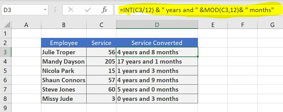
Hello Excellers, Welcome to another blog post in my #FormulaFriday #ExcelTips series. Today I will show you how to create a Month to Year calculator in Excel. I have a sample file below to work through. This extract is from a Human Resources database that exports the length of service in months. I would like to see this in Years and Months for convenience.
So, for the first record in the database, Julie Troper has a service value of 56 months. It is much more convenient to view the length of service in Years and Months, not just months.
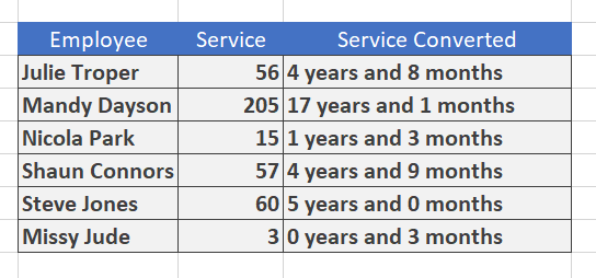
So, let’s insert a new column into the data set and calculate the Months into Years. The result will look like this screen grab below.
The Solution. Creating A Month To Year Calculator In Excel.
The solution uses the INT function and the MOD function. Let’s work though the calculation one step at a time.

The INT Function.
The Excel INT function returns the integer part of a decimal number by rounding it down to the integer. In the first part of this solution, the fifty-six months is divided by twelve months in the year to convert the months into years. So, Julie Troper will have served four years. Therefore, four years is the result of fifty-six months divided by twelve rounded down..
The MOD Function.
The second Excel function used in this solution is the MOD function which returns the remainder of two numbers after division. We already have the INT Function calculation for how many years, and this function will cover the remaining months. Right on!.
Putting It All Together.
The rest of the formula simply adds in the text Years and Months. How cool is that right?. Use “&” to join the results of INT and MOD to get the final result. You can copy the formula below if you need to. Just adjust the cell references for your Excel worksheet.
=INT(C3/12) & ” years and ” &MOD(C3,12)& ” months”


