I touched briefly on the MIN and MAX functions in my recent How To Excel At Excel Newsletter. If you want to sign up for 3 top tips every 15 days then just enter your email address here and as a bonus I will send you a link to a free e book with 50 TOP Excel tips…..
Here I want to look at these a bit more and combine them with some other Excel functions and turn up the heat…a little. The MIN and MAX functions I find great for quick little calculations of the MINimum and MAXimum values in a range of data.
For example the following function will find the minimum value in the range of cells G4:G19.
=MIN(G4:G19)
In this case it is €35566.00
At the opposite end of the scale the following function will find the maximum value in the range G4:G19
=MAX(G4:G19)
In this case the MAX value is €447177.00

That’s all well and good but let’s turn up the heat a little… and really put these two little functions to some real use. I have used the next examples in my work to find the maximum and minimum pricing of certain products charged by our Business Developers……handy.
OK, so we need to find the MINimum cost price charged for a product called W213.
Now then there is no MINIF function in Excel unlike SUMIF or COUNTIF, but we can easily combine MIN and IF functions to just do that ourselves and enter the formula as an array.
MIN IF formulas combined
First enter the MIN and IF functions with their appropriate opening brackets
=MIN(IF( ………..So far so good….
Next we select the area that contains the Pricing data charged. We can hit F4 to make the list absolute.
=MIN(IF($G$2:$G$28
Next type an equals sign = and click on the cell with the Sales Product List. This reference won’t be locked. As we will be moving down the cells the reference the different products
=MIN(IF($G$2:$G$28=B3
Then type a comma and select the cells that contain the pricing charged for the products -again press F4 to lock this range of cells.
=MIN(IF($G$2:$G$28=B3,$H$2:$H$28
Now we can finish up the formula ( my favorite bit) with two closing brackets. As we are dealing with an array, we hit CTRL+SHIFT+ENTER
{=MIN(IF($G$2:$G$28=B3,$H$2:$H$28))}

If you do not have the curly or array brackets then just put the cursor somewhere in the formula bar and press the CTRl+SHIFT+ENTER combo. All you need to do then is copy the formula down the rest of your cells to get the Minimum price of your products- Excellent huh?
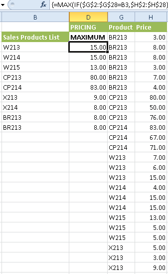
MAX IF formulas combined
First enter the MAX and IF functions with their appropriate opening brackets
=MAX(IF( ………..So far so good….
Next we select the area that contains the Pricing data charged. We can hit F4 to make the list absolute.
=MAX(IF($G$2:$G$28
Next type an equals sign = and click on the cell with the Sales Product List. This reference won’t be locked. As we will be moving down the cells the reference the different products
=MAX(IF($G$2:$G$28=B3
Then type a comma and select the cells that contain the pricing charged for the products again press F4 to lock this range of cells.
=MAX(IF($G$2:$G$28=B3,$H$2:$H$28
Now we can finish up the formula (my favorite bit :-)) with two closing brackets. As we are dealing with an array, we hit CTRL+SHIFT+ENTER
{=MAX(IF($G$2:$G$28=B3,$H$2:$H$28))}

If you do not have the curly or array brackets then just put the cursor somewhere in the formula bar and press the CTRl+SHIFT+ENTER combo. All you need to do then is copy the formula down the rest of your cells to get the Maximum price of your products…..
How cool is that?.
You can download the sample file to work with and explore the MIN and MAX Functions yourself-
Right Here


