Hello Excellers, welcome back to another #Excel #FormulaFriday blog post in my 2021 series of Excel formula tips. So, due to a colleague asking about the GETPIVOTDATA function (which seemed to cause some confusion) I thought it was time to walk through GETPIVOTADATA . I therefore will use a sample Excel Pivot Table. So, read on to solve the GETPIVOTDATA issue.

What Is The GETPIVOTDATA Function?.

Have you heard of the GETPIVOTDATA function in Excel?. If you look up the Function in the Insert Function area in Excel it is given a very straight forward explanation. It is categorised under the LOOKUP and REFERENCE Functions in Excel.

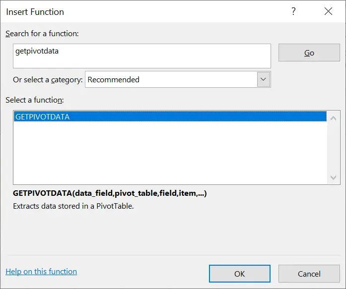
GETPIVOTDATA will extract, group, or add data from an Excel Pivot Table. Simple right?. We can query the Pivot Table and return specific data based on the Pivot Table structure instead of the cells references.

Syntax Of GETPIVOTDATA.

So, let’s take a quick recap of the syntax of the function.

=GETPIVOTDATA (data_field, pivot_table, [field1, item1], …)

Where

data field – this is the name of the value field to query

pivot table – this refers to any cell in the pivot table query

field1, item1 etc- this is a field item/pair. and is optional. Up to 126 pairs can be used.;

Working Through An Example.

I always find it is easier to work through an example right?. The link to the link the Excel workbook is below if you want to try this out yourself. So, click the link below to do that.

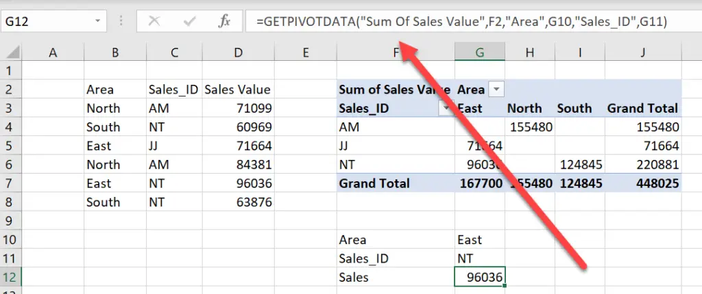
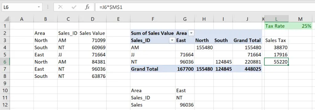
This is my sample data below. I have already created a simple Pivot Table from the data set. This represents sales data per area or region by Sales ID.

So, back to the GETPIVOTDATA function. The first argument (data_field) names a value field to query. The second argument (pivot table) is a reference to any cell in an existing pivot table.

Then, additional arguments are supplied in field/item pairs that act as filters to limit the data retrieved based on the structure of the pivot table.

So, for example, my formula in cell G12 is

=GETPIVOTDATA(“Sum Of Sales Value”,F2,”Area”,G10,”Sales_ID”,G11)

This, therefore, causes the function to retrieve data from the field “Sum Of Sales Value” in the pivot table that begins in cell F2. The data is limited to the area”East” for the Sales ID “NT”. The values for Area and Sales_ID come from cells G10 and G11.

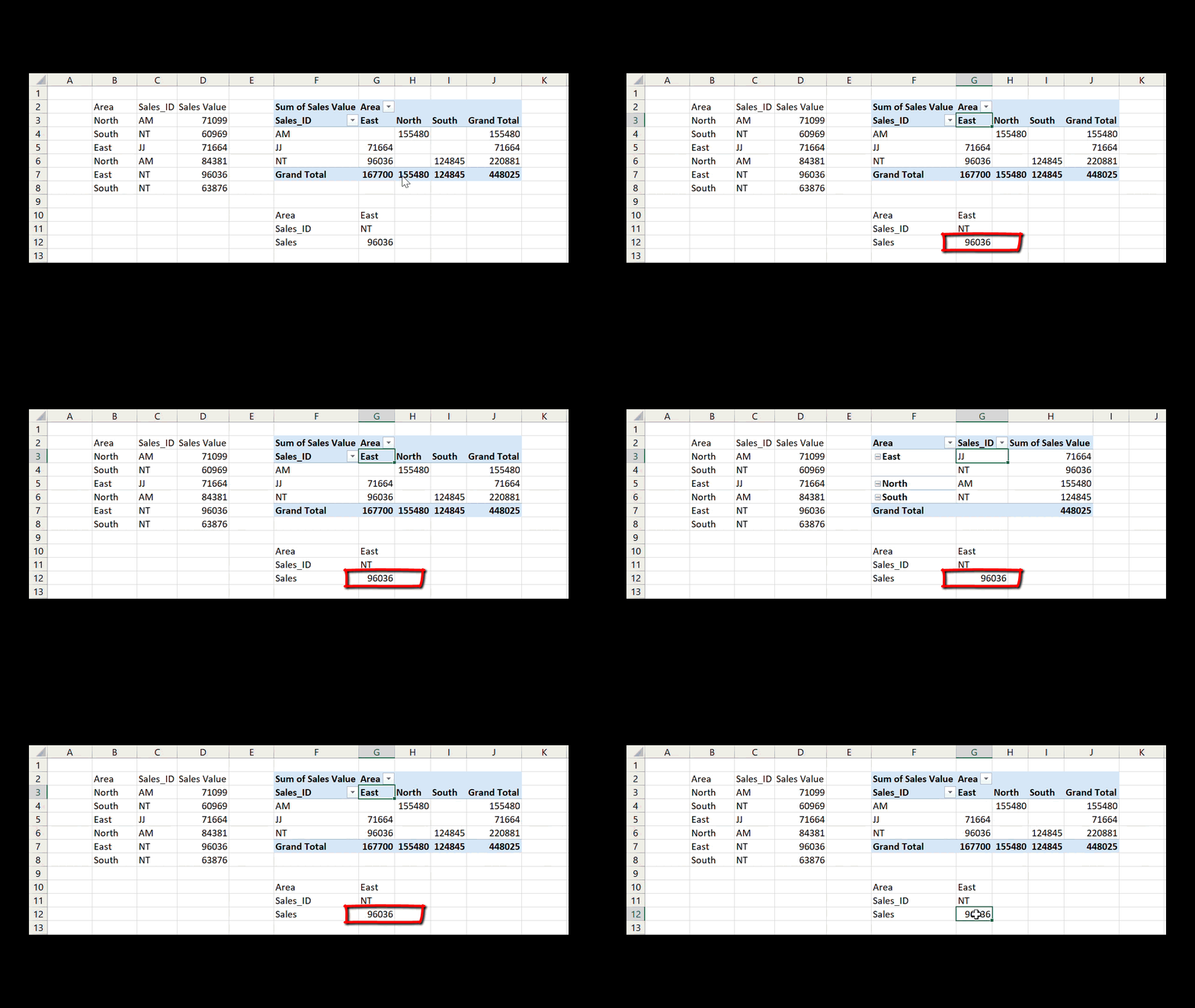
The GETPIVOTDATA function will continue to return the correct data even if the table changes. How Cool is that?????.

Possible Errors.

If the pivot_table argument is not a range in which a Pivot Table is found, GETPIVOTDATA returns the #REF! error. Also, if the arguments supplied do not describe a visible field, or if they include a report filter in which the filtered data is not displayed, GETPIVOTDATA returns the #REF! error value as well.

Turning Off GETPIVOTDATA.

Ok, so back to my colleague mentioned right back up there at the start of this blog post. They had found that when they tried to carry out a calculation based on their Pivot Table, the formula was not exactly behaving as expected.

They were trying to calculate sales tax on their sales values. In fact, there are a number of ways to do this with a Pivot Table.

• Use a calculated field.
• Write a simple formula in the adjacent cell. (This option is discussed below).

As a result of the formula being used the output can be seen in the screen grab below. The second method was being used. The simple formula. The formula was not filling properly as they dragged the formula down. It was not behaving as expected. The tax rate is stored in cell M1 at 25%.

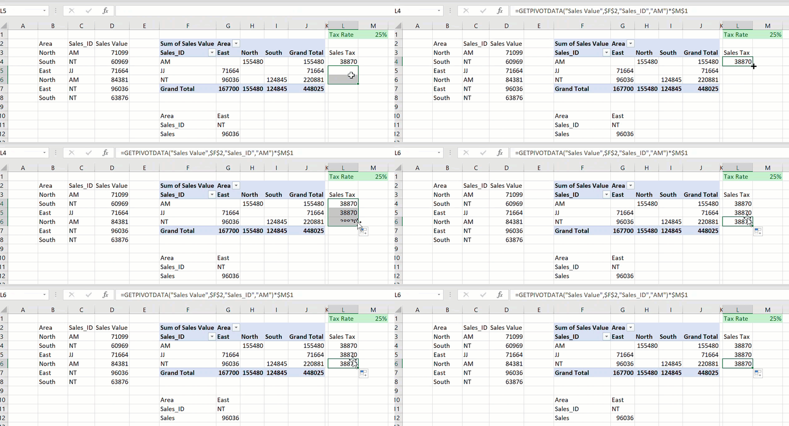
The formula cannot be dragged to replicate it to other cells as GETPIVOTDATA, in this case, is enabled. Therefore it needs to be disabled.

• Hit ALT F+T
• Formulas | Working with formulas
• Then, un-Check the GETPIVOTDATA function
• Finally, job done

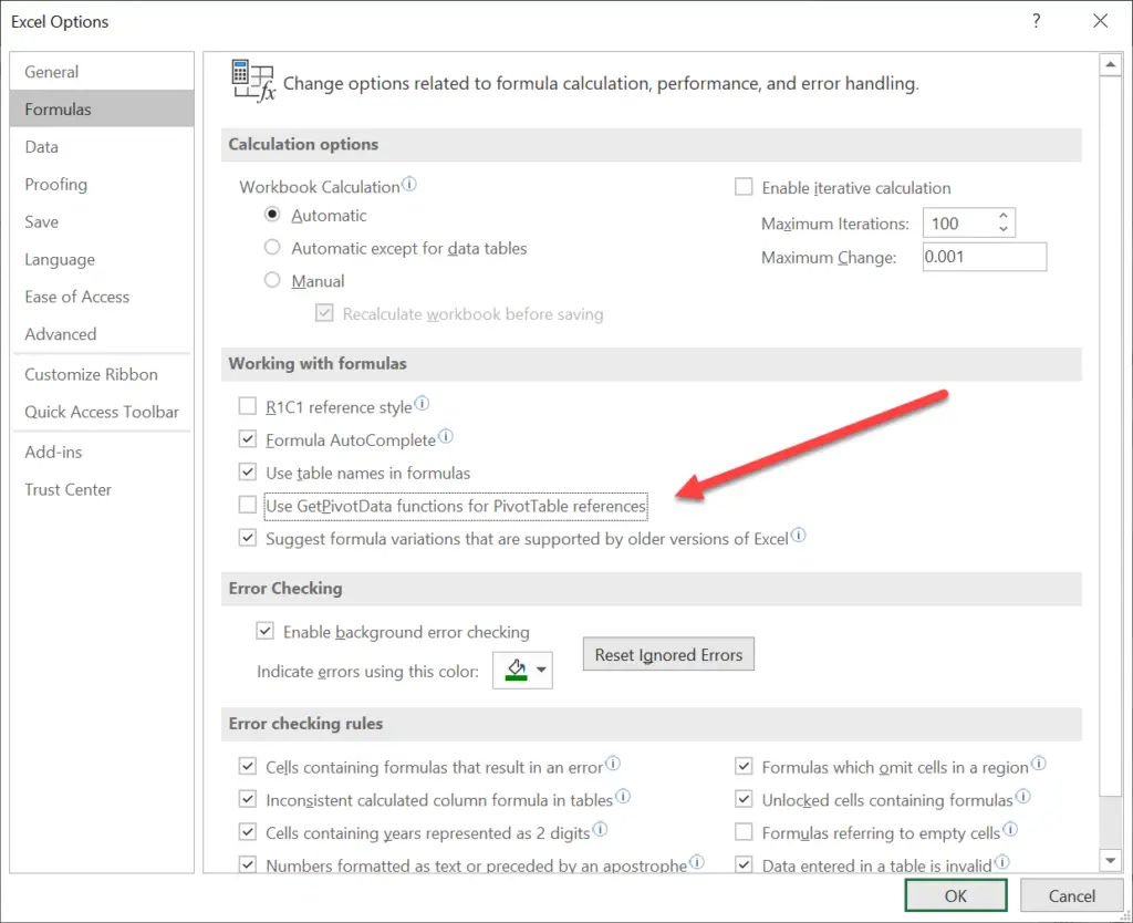
The formula is now working as expected again with the formula moving down when dragged as expected.

So, if you want more Excel and VBA tips then sign up for my Monthly Newsletter. I share 3 Tips on the first Wednesday of the month. You will receive my free Ebook, 30 Excel Tips. Do not forget to check out all of my Formula Friday blog posts below.

Finally, I have teamed up with Excel Rescue to help solve ANY Excel problems. So, why not click the link and take a look?.