Hello Excellers and welcome back to another #Excel #FormulaFriday blog post in my Excel 2020 series. Today I want to show you how to not only hide your Excel formula from users but lock those cells. This will prevent any user from attempting to edit your formulas. Keep your hard work away from prying eyes right?.
Note. I am not claiming this is 1oo% foolproof but will prevent the average Excel Joe user busting out your Excel Dashboard, or worksheet solution.
If you have created a great Excel dashboard or Excel solution then chances are you do not want any users tinkering around with it. You worked hard on it right?.
Step 1. Unlock All Cells In Your Worksheet.
So, I know this sound absolutely nuts. You want to hide and protect all of your Excel formulas. But, the first stage in this process is to unlock your whole worksheet. Trust me.
All cells by default are flagged as Locked by default. Just select any cell or range of cells in your Excel worksheet. We need to set all cells to unlocked to begin our process.
- Hit Ctrl+A to select all cells in the worksheet
- Use Ctrl+1 to to open up the Format Cells dialog box
- On the protection Tab un-check the locked option.

This has set up up nicely to hide our formulas and lock the cells.
Step 2. Find All Cells With Formulas.
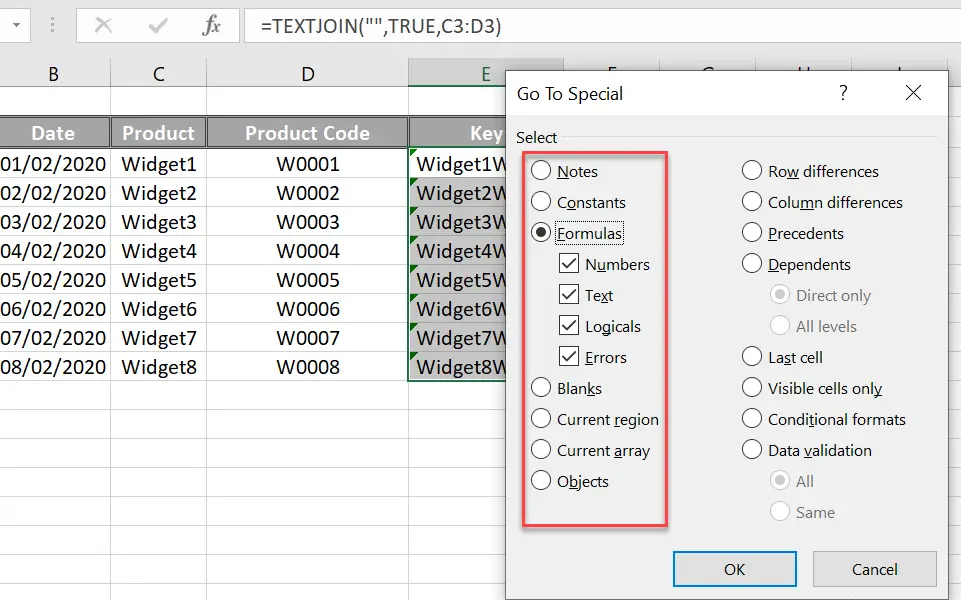
So, the next step is to find all of the cells in our Excel worksheet that have formulas. There is a quick and easy way to do this. We use the GoTo Special feature.
All of the cells in your worksheet should still be selected after step 1 above is completed. Now follow the simple steps below.
- Press F5 to open the GoTo Special dialog box.
- Click Special
- Select Formulas
All of the cells that contain formulas will be selected and highlighted. This is so useful if you have a really big Excel worksheet. Not all the worksheet cells are visible at once. This method will mop all cells with Excel formulas.

In my simple example you can see that cells E3 to E10 contain TEXTJOIN formulas. These are the only formulas I have in my worksheet. But, if I had non contiguous formulas, be assured the GoTo Special feature would pick them all up.
Step 3. Hide Excel Formulas And Lock Cells.
So, for next step, now we have all cells with formulas selected is to hide those formulas.
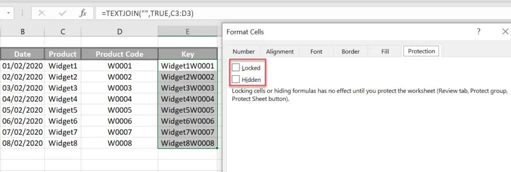
All Excel cells have two attributes, that of locked and hidden. Locked cells are just that, locked and cannot be changed by an end user, whereas the hidden attribute means that formulas contained in those cells will not be displayed in the formula bar at the top of the worksheet.
- Use Ctrl+1 to to open up the Format Cells dialog box again, as the cells with formulas should still be selected from the previous step.
- On the protection Tab tick both the Locked and Hidden boxes.
- Hit Ok to close the dialog box.

We do however need to also remember that none of these attributes are in force until a worksheet is protected.
Step 4. Protect The Worksheet.
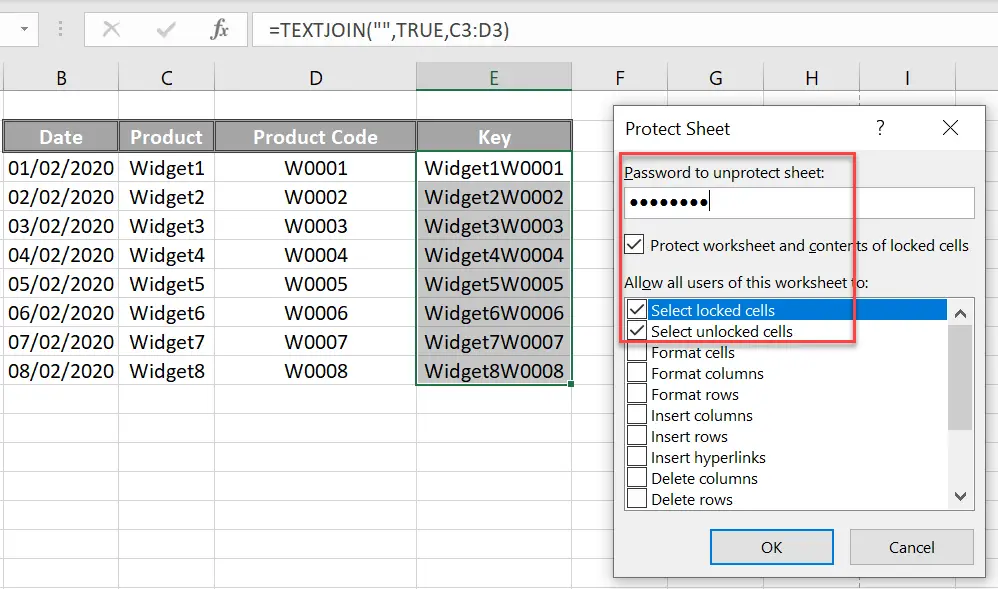
The final step is to protect the worksheet and the settings we have selected for our cells that contain formulas.
- Hit the Review Tab
- In the Protect Group select the Protect Sheet option.
- Ensure that Protect Worksheet and Contents are selected
- Enter a Password when prompted.
- Job Done!
This password is needed for unprotecting the worksheet. No one, even yourself, will be able to edit the sheet without entering the password, so do remember it.

So that is how to hide Excel formulas and lock the cells to avoid users editing your hard work!.
So, if you want more Excel and VBA tips then sign up for my Monthly Newsletter. I share 3 Tips on the first Wednesday of the month. You will receive my free Ebook, 30 Excel Tips.
Other Excel Tip Blog Posts You May Like
Formula Friday -Delete Values From Cells While Keeping Formulas
Formula Friday – Setting Excel To Calculate Formulas Manually
