Excellers, it’s time for more Formula Fun.

Today I am going to show you how to use the approximate match in the VLOOKUP formula to apply Grades such as A,B,C,D etc to student papers dependant on the marks on their paper. So for example all papers with a grade of 70 or over should receive a Grade A etc.

So firstly we need to set up our grades table as below………

The Paper Scores need to be sorted in Ascending Order.

 

We can now go ahead and wrote our VLOOKUP formula, and when we get to set the final argument, set it to TRUE or you can also leave this blank to search for the nearest match.  With non-exact or neareast matches, VLOOKUP moves to the first value that’s higher than the lookup value, then falls back to the previous value.

 

 

=VLOOKUP(E12,$C$3:$D$7,2,TRUE)

Our Formula reads like this……..

Lookup the value in E12 in the range of cells C3 to D7 (this is made absolute so when we drag the formula to reast of the scores we want to grade the lookup formula looks in the correct range of cells).  We want to return the matching value in column 2, and we set the final argument to TRUE for an nearest match. Simple as that.

 

It’s important to remeber that if you allow non-exact matches with VLOOKUP, you must make sure that your table is sorted in ascending order.

 

Want to Learn More Formulas?

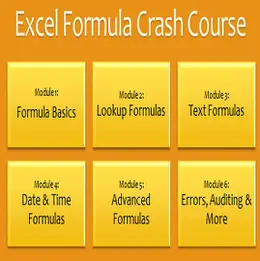
Join the Excel Formulas Crash Course.  If you want to learn SUMIFS, SUMPRODUCT, OFFSET and 40 other day to day formulas, then consider Chandoo’s Excel Formula Crash Course.

It has 31 lessons split in to 6 modules and makes you awesome in Excel formulas.