 Hey Excellers, one of my favorite times of the week, #formulafriday time!. Today let’s look at avoiding Excel displaying a negative number after a calculation of stock items in an itinerary.
This again is another discussion I had with an Excel user recently, they only needed Excel to display a zero (rather than the actual negative value) if the result of the calculation of stock in and out resulted in a negative value.
So, let’s flex our formula fingers, as there were a couple of ways that we could so this. Here is an extract of the data from the warehouse.
Method 1. Use The IF Function.
The first method uses the IF statement, which can have one of two results, one if your statement or comparison is true, the other if it is not.
So we want to state if the result of the formula (Stock Out – Stock In) is less than 0 to return a zero, and if it is not less than 0 then give then simply return the result of the formula.
It looks like the output below –
We can see that the second and fourth line of our stock balance formulas will have resulted in a negative number, so instead we have chosen to instruct Excel to return zero instead. This is pretty straightforward logic and does the job.
Method 2. Use The MAX Function.
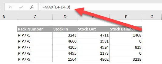
There is another way to carry out the same process. We can use the MAX function in Excel which returns the largest value in a set of values. The Syntax of the MAX is
MAX(number1, [number2], …)
Only the first number is required, subsequent are optional.
So by setting the first value as the result of the formula E4-D4, and the second number as zero we will never display a negative number as the zero will be the largest number if indeed a negative number is calculated as a result of the formula. Clever huh?. It looks like this.
Two easy methods to display zero instead of a negative value.
If you want more Excel and VBA tips then sign up to my monthly Newsletter where I share 3 Excel Tips on the first Wednesday of the month and receive my free Ebook, 30 Excel Tips. If you want to see all of the blog posts in the Macro Mondays Series you can do so by clicking on the link below.


