Hey, Excellers time for more Friday Formula Fun.

Today let’s look at how to deal with the #N/A error we get when no match is found when using VLOOKUP. It’s a handy error as it tells us when there is no match, but does not look great, how about we mask it somehow or replace it automatically with something else.

We can do just that with the IFERROR function. An example work through?- of course.

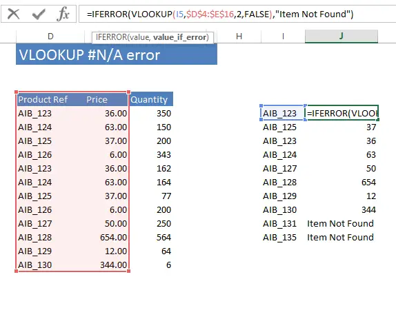
I have set up the typical VLOOKUP function to look up the price of products. All is good until the last two records which are not found. (AIB_131 and AIB_135). We get the default #N/A.

Let’s treat this a bit different by adding a little extra to the formula and tell Excel to return Item Not Found instead of the #N/A.

The amended formula looks like this

=IFERROR(VLOOKUP(I5,$D$4:$E$16,2,FALSE),”Item Not Found”).

All we do is use the formula IFERROR(Value, Value If Error) and wrap it around the VLOOKUP formula.

The result of the VLOOKUP is not affected if there is no error, but if an error is a the result Excel indeed will return “Item Not Found”. You can of course replace the example text with your own or indeed with numbers of characters of your choice.