Happy Friday Excellers. Today I want to share with you how to RANK a data set with the rank formula in Excel, but ignore zero values. I use RANK a LOT, and sometimes you just do not want to include zero values in your results. When you are working with large data sets in Excel, sorting and ranking your data can be a helpful way to narrow down your focus. However, when you have zero values in your data set, it can be tricky to determine where your data should be ranked. In this blog post, we will show you how to use the RANK function in Excel to ignore zeros and rank your data accordingly. Let’s get started!
Rank Excel Formula Ignoring Zeros
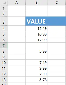
We actually are going to make use of the IF function as well as RANK Excel function in this solution. Here is sample data set I want to rank.
I have 10 lines of data and 2 of them are zero. I do not want zeros to be included in the ranking values or calculations. This is the formula I am using to achieve this.
=IF(B4=0,””,RANK(B4,$B$4:$B$13,0))
Let’s Walk Through The Formula.
If B4 contains a zero then Excel returns a blank cell “”. If the value in in cell B4 is not equal to zero then the value is ranked in the cell range of B4 to B13. This returns the ranking of 2. We can then drag the formula down the length of the data range to populate the whole data set.
I hope you found this tip on how to use the Rank Excel Formula. See you next time for more #FormulaFriday fun.
Dont forget to sign up to the Excel at Excel Newsletter for 3 free Excel tips . I send out these tips every month. Just click on the Sign Up Form to the right or use the link below.


