Hello Excellers Happy Friday and it’s time for some more #formulafriday fun. Today let’s look at how to use the ISFORMULA function to achieve the following
- To test a cell reference to see if it contains a formula
- Conditionally format a cell reference if it does contain a formula.
This is really useful if you need to see all of the cells that contain formulas at once on your Excel worksheet.
You could use the GOTO option in Excel, but in this way you can highlight your formulas containing cells on a more permanent basis.
ISFORMULA Syntax
ISFORMULA has the following syntax.
ISFORMULA(reference)
Where
reference – this argument is required. It is the reference to a cell you want to test. It can be a cell, formula or a name that refers to a cell.
(note – if the reference is not a valid data type (such a s defined name) then Excel will return the #VALUE! error
Example 1. Test A Cell Reference To See If It Contains A Formula.
ISFORMULA will return TRUE if there is a formula in an Excel worksheet cell (and FALSE) if not. Using the example in my worksheet below. I typed the formula =ISFORMULA(D5) and dragged the formula across to F5.
I can see that cells D5 and E5 do not contain a formula (FALSE has been returned), but F5 does as the result has been returned as TRUE.
So, lets move on and use ISFORMULA to highlight cells with a formula with some conditional formatting.
Example 2. Conditionally format a cell reference if it does contain a formula.
In this second example I have a small sample of data that calculates the ranking of sales for five stores. Follow these simple steps to highlight the cells in the data set that contain formulas.
- Select your data set, in this case it is cells D10:F11. Ensure that the first cell in the data set is selected as the active cell.
- Home Tab – Styles Group – Conditional Formatting
- Select New Rule
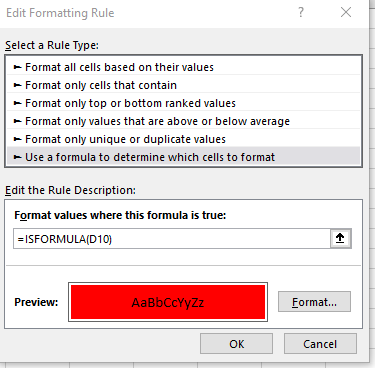
- Click use a formula to determine which cells to format
- Enter the ISFORMULA in the dialog box and refer to the active cell, in this case D10
- Click the format button and select the type of formatting you want to apply, in this example I have chosen red
- Hit Ok twice to apply the formatting rule
- Only the cells with formulas will be formatted as red
- Excel has correctly identified cells F10 and F11 and containing a formula
If you want MORE Excel and VBA tips then sign up to my monthly Newsletter where I share 3 Excel Tips on the first Wednesday of the month and receive my free Ebook, 30 Excel Tips. If you want to see all of the blog posts in the Macro Mondays Series you can do so by clicking on the link below.


