Hey Excellers it’s Formula Friday and also Happy New Year!…. Let’s look at using the dollar $ sign today in formulas and fixing cells references.

As you probably know formulas refer to cells, and when they refers to a cells a cell reference is used- for example cell A1. There are three types of cell references in Excel – Relative, Absolute and Mixed.

Relative Cell References– With these type of cell references, when you copy or moved a formula to a cell other than which the formula was entered then then the cell references change relative to the new position.

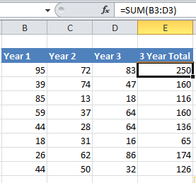
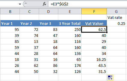
The row and column portions of the formula are not preceded by the $ sign. For example for example, A1 is a relative reference to cell A1. If moved or copied, the reference changes by the same number of rows and coulmns as it was moved. So, if you move a formula with the relative reference A1 one cell down and one cell to the right, the reference changes to B2 . As we know this type behaviour is very useful and is what allows a formula to be copied across or down the page and automatically refer to the new column or row that it finds itself in. See the example below- we can drag the formula = Sum(B3:C3) in D3 right down the column to D10 and formulas. Absolute Cell References – In some situations you may want the cell reference to reman constant or what is called absolute. This is where the $ is used. Using our previous example, let’s calculate Vat Value of the 3 Year Total Value. We can store the value of the VAT rate in a cell G2 then refer to that cell in our formula as below. If we were to just drag the formula down the column of date as in our first stage of this example, then then the formula would not work as the cells will move down as the formula is dragged- not what we want. This is where the dollar sign ($) is used. The dollar sign allows you to fix either the row, the column or both on any cell reference, by preceding the column or row with the dollar sign. We want both to be locked so any way we drag a formula the Vat Rate remains a static cell. In our example if we replace the formula in cell F2 with =E3*$G$2, then both the G and the 2 will remain fixed when the formula is copied. Just what we want.
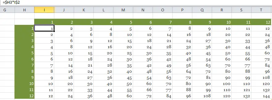
Mixed References -these are exactly that a mix of either the column or the row being fixed. The best example of this is to look at times tables where we want to every cell in the white area to be the product of its row and column heading. Easily achieved with a mixed cell reference using the $ correctly
In cell B2, the formula without dollars would be H3*I2, but for this formula to work when copied to each column, we need it to always look at column H for the first reference and to work for each row, we need to always look at row 3 for the second. Using the dollar sign to do this, it becomes =$H3*I$2. This can then be copied to every cell in the white area as below –

Don’t forget the quickest way to enter the $ sign is to hit the F$ key when entering the formula. By repeatedly hitting the F4 key, toggles between no dollar signs, both dollar signs, just the row and just the column.