Download the practice File

[ddownload id="7090"]

Hello Excellers yet another week has gone and let’s finish it with another Formula for Friday.

Today we are diving into the arena of the Array Formula with a simple straightforward example where I will show you how to quickly calculate the most improved sales area from one month to the next.

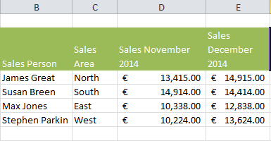
In our example we have four sales areas, looked after by four sales people.

North, South, East and West Sales for two months- November and December 2014- let’s see which areas had the most improved sales using both the November and December sales figures.

Without using an array formula we follow the steps below to find the most improved sales area.

1. Calculate the improvement (if any) of each of the sales area in column F by subtracting December 2014 sales from the November 2014 sales figures using the formula below-

2. We then need to use the MAX function to find the maximum value and therefore the most improved sales.

We can see that Stephen Parkin has the most improved sales for the West area. But that took us two formulas, there is a quicker way.

Use An Array Formula

If we were to use an array formula, we can use Excel to perform the multiple calculations in just one cell for us. We do not need to store the range of values in Column F as Excel can store this in it’s memory. This is called an array constant. So let’s repeat the process by

1. Starting with the MAX function

=MAX(

We then want to replace the E3 with E3:E6

and then replace D3 with D3:D6

with a result of the formula looking like this

=MAX(E3:E6-D3:D6)

2. To indicate the Excel this is an array formula we need to surround it with curly braces or brackets { }.

We do this by instead of hitting return after the formula is typed hold down CTRL+SHIFT+ENTER. I usually ensure my cursor is in the formula, then hold down CTRL+SHIRT then hit ENTER until you get the hang of it!.

So the MAX function is using the array constant as an argument and results in € 3,400.00.

Extra Tip

When you are working with array formulas, you can take a look at the array constants yourself. Using the same example.

1. Select the cell referencing that relate to your array in your formula.

2. Hit F9, you no see what Excel sees.

3. Elements in a vertical array constant are separated by semi colons and horizontal ones are separated by commas, in our example it is of course a vertical array constant so are separated by semi colons.

I hope you enjoyed Formula Friday. Don’t forget to Comment, sign up and follow for more Excel Tips with my Social Media Links right here below.

Want To Watch The Video Tip?

Download the Example file here

[ddownload id="7090"]