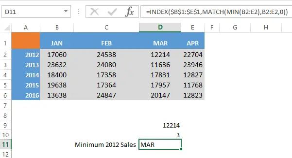
Today’s #formulafriday Excel tip will show you how to identify the the highest or lowest value in a row of data and return the column heading or title. So let’s say you have some data set out as below. Column A is our Year value and Columns B onwards are our months of the year values.

We can easily get Excel to return the highest or the lowest value month for each year with a few clever functions. That’s what we are here for Formula Friday fun!!!. The formula or functions we are going to use are……..INDEX (one of my absolute favourite functions) and MATCH combined with MAX and MIN. Let’s get started!
So what does INDEX do?.
INDEX returns the value at the intersection of a particular Row and Column, or it allows you to look up a cell in a column or table of data and return the contents of that cell. The Syntax of INDEX is
=INDEX(array,row_num,column_num)
array– this is the range of cells you want INDEX to look in.
row_num – this is the ROW you want INDEX to look in. This is a number or you can use a formula to find the number you want.
column_num refers to which COLUMN you want INDEX to look in, it’s optional and only needed if you want to look anywhere apart from the first column of the array you specified.
So What does MATCH do?
MATCH searches for a specific items in a range of cells and returns the relative ppsotion of the item in that range.
=MATCH(lookup_value,lookup_array,[match_type])
lookup_value– this is required in the function and is the value value you want to lookup in the lookup_array.
lookup_array – this is required- it is the range of cells to want to search.
match_type -this is optional. The match_type argument specifies how Excel matches lookup_value with values in lookup_array. The default value for this argument is 1.
A match type of 1 is the largest value that is less than or equal to the lookup_value- this is the default even when ommited.
A match type of 0 finds the first value that os exactly equal to the lookup_value.
A match type of -1 finds the smallest value that is greater than or equal to the lookup_value.
So what does MAX and MIN do?
Max finds the highest value in a range of cells and MIN finds the smallest value in a range of cells.
Ok let’s see how all of these fit together to get our correct results from our example looking at the values for the year 2012.
=MIN(B2:E2) this returns the answer 12214 being the smallest value in 2012

=MATCH(MIN(B2:E2),B2:E2,0) this returns 3 as this is the position of the lowest number in our row

We now know the position of the lowest value, lets add in the magic piece we need…. to return the Month in our header rows which corresponds to that lowest value.
So, we finally hit up the formula with the INDEX funtion.
=INDEX($B$1:$E$1,MATCH(MIN(B2:E2),B2:E2,0))

There we are March had the lowest sales in 2012. If we want to find the highest or MAXIMUM sales we just use MAX in replace of MIN in the formula.
- Create A Micro Chart In Excel
- How To Display a Plus + Sign On Positive Numbers With Custom Formatting In Excel
- Create A Timestamp In Excel With Formulas
- Use TRIM for a speedy data clean up


