Friday Formula time….. Today let’s look at a handy formula for transforming an email address into a name, without the email address junk that is associated with it.
At work I get data extracts that include email addresses rather than system usernames. In order to carry out my analysis I have to extract the username from the email address that is logged in the data extract. It is straightforward by using the LEFT and FIND functions.
See a small extract of my data set below.

So let’s dive into the formula starting with the LEFT function which allows you to extract a substring from a string, starting from the left-most character
The Synatx of LEFT is
=LEFT(text,number_of_characters)
WHERE
- text – The string that you wish to extract from.
- number_of_characters – this is optional. It indicates the number of characters that you wish to extract starting from the left-most character. If this parameter is omitted, only 1 character is returned.
The next part of the formula uses FIND function returns the location of a substring in a string. The search is case-sensitive.
The Syntax of FIND is
=FIND(substring, string, start _ position)
WHERE
- substring – this is substring that you want to find.
- string – this is the The string to search within.
- start_position – this is optional. It is the position in string where the search will start. The first position is 1.
So let’s put it all together!
Starting with the LEFT function to reference the first cell with our text data – B3 and we want to extract information from the begining of our cell.
=LEFT(B3,
We then need to put in the number _of_characters, but they will be all different lengths…so this is where we use the FIND function to find @ in our text string and return the number character that it is….
=LEFT(B3,FIND(“@”
We then need to tell FIND to look for the “@” symbol in B3
=LEFT(B3,FIND(“@”,B3
And to start looking from the first character
=LEFT(B3,FIND(“@”,B3,1)
After closing the brackets, we then finish off the formula by typing the -1 in the formula as the last character we want is the one BEFORE the “@” symbol
=LEFT(B3,FIND(“@”,B3,1)
Hit ok and test it!

Double click and populate the full data set with the formula.
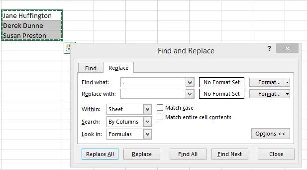
All well and good, we could leave the name with the . in between the first name and surname. But if you want rid of those as well, we can use the Find And Replace functionality in Excel to remove it.
- First select your newly extracted names
- Hit Copy (CTRL+C) and then Paste Special Values
- Select your new names again
- Hit CTRL+F in the find enter .
- In Replace With hit the spacebar
- Select to search by COLUMNS
- Hit Replace All

Job well done!. A clean data set ready for some analysis!


