One of the most basic Excel function new users learn along with SUM, COUNT and MIN is the MAX function.  However, in previous Excel years- 2003 and earlier, you had to actually type the MAX  formula! What you saying?.

Yes that’s right you had to type the MAX formula to find the maximum or largest value in your range. If you still want to go old school then you can and go ahead and type your formula.  Here is an example.

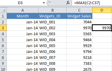
D3 contains the formula to find the MAXimum of widgets sold in the last 6 months.

 

=MAX(C2:C37)

 

 

 

 

 

 

 

 

Life is way easier now and we had the fabulous auto sum drop down box in Home Tab – Editing Group

 

This is all pretty simple stuff, so let’s turn up the volume a bit here and when we combine the MAX function with the IF function we can actually create a conditional MAX-IF formula which adds a great twist and power to our function.  We can now find the largest value in our range of numbers (in our example the number of widgets sold) that actually meet conditions that we specify.

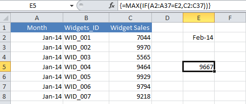
For example instead of just getting Excel to tell us the Maximum number of widgets sold, we can specify the maximum numbers of widgets sold with a criteria of Feb 14.  So we are asking the question, what is the maximum numbers of widgets sold in February 2014. Let’s build the formula using the two in built function in Excel- Max and IF.

We first begin with =Max(If(  

………we include both functions with their own opening brackets.

Next, we want to find the rows where the Month of Feb 14 matches which we have stored in cell E2

=Max(If( A2:A37=E2,

If the date matches we then want to test the quantity of Widget Sales, we then close the two sets of brackets.

=Max(If( A2:A37=E2,C2:C37))

As this is an array formula we need to enter it as an array by hitting CTRL+SHIFT+ENTER

{=Max(If( A2:A37=E2,C2:C37))}

That’s it we have not only used the MAX function but combined it with the IF function to get real valuable information easily form our Excel data.