Hello Excellers, welcome back to another #Excel #FormulaFriday blog post. In Excel, some formulas are quite complex, while others are simple. This blog post will focus on the EXACT formula in Excel. The Exact in Excel compares two text strings and returns TRUE if they are the same and FALSE otherwise. EXACT is case-sensitive but ignores any formatting differences. I will show you how to use it and provide some examples. Stay tuned!
How To Excel At Excel – Formula Friday Blog Posts.
Exact Excel Synyax And Example.
So, let’s look at working through a simple example. But first, a quick refresher of the syntax of the Exact Exel syntax.
=EXACT(text1,text2)
Where
- text1 – The first text string to compare.
- text2 – The second text string to compare.
So all we need to do is supply two values to compare. Excel will find an exact match and return the value TRUE. If they are not an actual match, Excel returns the value FALSE. (This function also works with other numbers and logical values). Let’s walk through an example as usual.
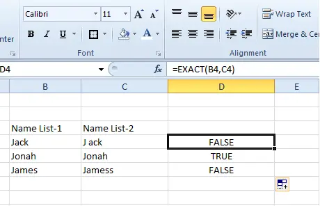
We have two sets of data in columns B and C. We want to see if the same value is in B and C equivalent cells. So let’s go ahead and write the formula
=EXACT(B4,C4)
We can quickly identify which two name lists are an exact match. The Exact Excel function IS case sensitive but IGNORES formatting. Let me know if you use this formula in Excel.
More Excel Tips


