Hello, Excellers. Welcome back to another blog post in my #FormulaFriday series. Today it is back to basics exploring the Rank function in Excel. The rank Excel formula will compare numbers to other numbers contained in an Excel list. So, if you apply the rank formula to a list of numbers, Excel will apply a ranking number to each number. This is either in an ascending or descending order.

Excel Rank Formula. Recap Of Syntax.
There are a few arguments for the rank function. Let’s do a recap.
=Rank( number, array, [order] )
number – this is the number to find the rank for
array – this is the range or array or number to use for ranking
order– this is an optional argument and it specifies how to rank your numbers
Notes on the order argument.
- Set the order value to 0 to rank the numbers in descending order.
- Set the order to 1 and the numbers are ranked in ascending order
- If the order argument is not supplied then if defaults to 0 (descending order)
A Rank In Excel Exmaple.
So let’s take a look at an example. I have generated league table for sales representatives. The league is ongoing based on their value sales that runs over the summer months. This seemed to be the ideal scenario to use RANK in Excel.
The data set is below. May 2016 already filled in as those sales figures are confirmed.
My league table consisted of 10 sales people in the department. They are ranked based on their sales volumes, from 1 to 10. One being the top ranking and ten the bottom. They are to be ranked over a three month period, May June and July.
I have added a column into the league which gives a total of all three months. This will be the basis of the rank. This way I only need to use the Total Sales column to use for ranking values. So, as we have the first months data let’s see how the Sales people are doing in their ranking up to now. Start by entering the =RANK function to begin the calculaton.
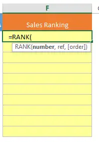
Starting The Solution.
So, begin with the first number to rank which is in cell reference E2. This is the number argument of the function.
Next, select the full data range of which to rank the number – $E$2:$E$11 – this is the ref argument of the function. Make this range of cells absolute with the $ so the formula can fill the whole column.
I want the ranking to be in descending order, so I have set the [order]argument of the formula to 0. (The highest sales are ranked 1 and the lowest 10).

Drag the formula to the full list cells. The Sales people are now ranked for May 2016 with Scott Chalmer in the lead. Well Done Scott!!!.

Once the sales figures for June and then July are updated, the formula automatically updates the ranking of the Sales people.
Finally, if you want to download the sample workbook to work through the example you can do so here.

Why not bookmark the Formula Friday and Macro Monday blog post pages. I update them every week. For three free Excel tips do not forget to sign up to my monthly newsletter. No spam. All free.