Hello Excellers and welcome to another #Excel #formulafriday blog in my 2020 series. Today I want to address an issue that happens a lot with Excel workbooks that have become too large and complex. So, have YOU got a big workbook with lots of Excel formulas that take a long time to calculate? Well, then you may well find this blog post very useful.
Have you Got This Excel Issue?.
When you are waiting for an Excel workbook to recalculate, a number of minutes may not seem a long time in the normal course of a workday. But, if you want to open a workbook, change a few cells then recalculate. Well, it can feel a LONG time. Especially if you are testing a new formula or calculation method in your Excel workbook.
Here Is A Solution.
But here is a great way to refresh a formula on only a selected number of cells in your Excel workbook, instead of recalculating all of the formulas in the spreadsheet.
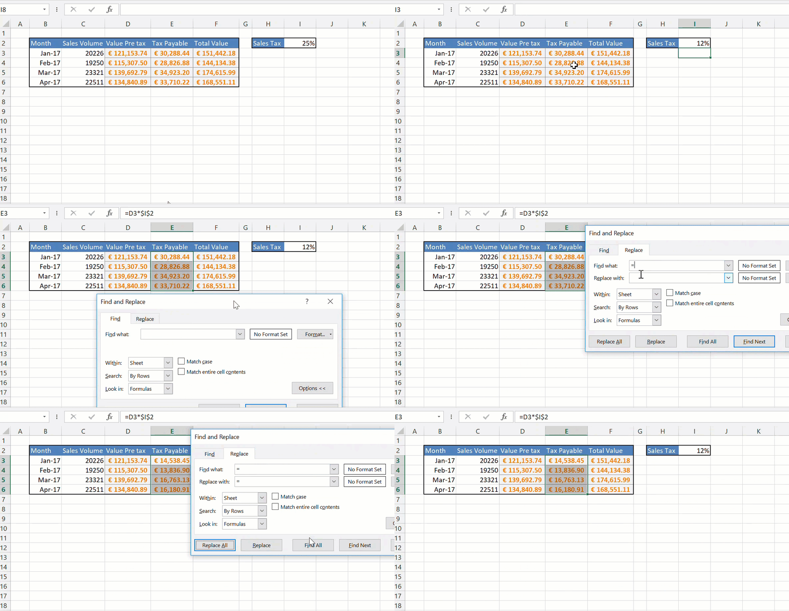
Let’s walk through an example. This is only a small sample data set, but it will show you how to use this great little hack Excel hack. I have a sample data set below. Very simple sales volumes and their pre and post-tax values with a specified tax rate in Cell I2.
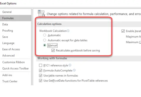
- First, switch to manual calculations
- File | Options | Formulas
- Calculation Options | Workbook
- Calculations | Manual
The Theory Behind This Method Of Calculation
Did you know that in Excel if you press F2 then Enter on a cell, only that single cells recalculates?. Yes, this will force a single cell to calculate. So certain cells can be calculated on an Excel worksheet. So, what if we combined this with a way to select specific cells. How about finding cells in a range (that we specify) by using Find & Replace.
So, let’s try to calculate Column E ONLY in our example data set only by changing the tax rate from 25% to 12%.
- Change the tax rate to 12%
- Select the cells that you want to recalculate
- Hit CTL+H to display the Find and Replace Dialog Box
- Type the = sign into the Find What box
- Type the = sign into the Replace With box
- Select the Options button and ensure that the Look In is set to Formulas and that match Entire Cell Contents is NOT selected (we are only looking to find the = sign)
- Click Replace all
ONLY THE SELECTED CELLS ARE CALCULATED.
As you can see in the screencast only the selected cells have been updated with the new 12% tax calculation.
This is really useful if you have a few cells you want to test with some new calculations without updating your whole worksheet and being stuck in a calculations loop.
Want to watch the YouTube video of this Excel Tip?.
Don’t forget the Subscribe and Hit The Notification Bell to be notified when my videos are uploaded.
If you want more Excel and VBA tips then sign up to my Monthly Newsletter where I share 3 Excel Tips on the first Wednesday of the month and receive my free Ebook, 30 Excel Tips.
If you want to see all of the blog posts in the Formula Friday series you can do so by clicking on the link below.
How To Excel At Excel – Formula Friday Blog Posts.


