Welcome back to another Excel #formulafriday blog. Today I want to share with you a nice handy Excel tip using a well-known formula. Let’s learn how to insert the contents of an Excel cell into a sentence. This is a really great way to save time if you use the same report every week or month. All you really need to do is update the report with the latest figures!.

Let’s walk through an example of my Monthly Sales Report. Every month I report on Sales Per Region, the standard format is the same every month and the only thing that changes is a handful of cells. Let’s free up some time and get this report a little more automated using the CONCATENATE Function.

Using The CONCATENATE Function.

The syntax of this formula is

=CONCATENATE(TEXT1,TEXT2…)

Up to 255 text entries can be added to the function and each one of them should be separated by a comma.

One point to note, CONCATENATE does NOT add in extra spaces between text, in order to do this, you need to accommodate these extra spaces within the formula. Let’s take a look at an example.

Right, let’s get back to the extract from my report-

Next, all I need to do is combine the text in cells B5:B8 with my monthly sales figures which are automatically updated on the datasheet of my Monthly Sales Report. You can be see these in the screenshot below. My sales figures I want to always refer to in the specified area of my Sales Report are contained in cells C6:C9.

As you have probably noticed we have some formatting on our cells that contain our sales figures for the previous month. So, I need to take into account this formatting for the sales report to not only look good but be easily interpreted.

Let’s get on with some formula fun.

First, we take CONCATENATE which simply combines two or more text strings into one. After that, we just need to separate the text strings with commas.

Building The Formula.

Let’s start with the Northern Region. We have three text strings as even space is classed as a separate text string. We also have to just ensure we force the formatting on the value sales from our data area of the Sale Report.

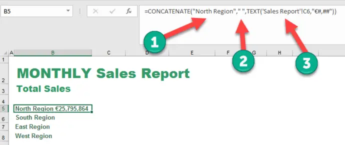
For the last argument (3) in the formula, we use the TEXT function, which takes two arguments. Firstly, it takes the Value (which we take from our data area of the sales report). We can then declare which formatting we want to use. I just need to hit enter to complete the process.

Now we have the formula set up. I just update the data area of my sales report. That’s all that I need to do. Excel automatically populates the presentation part of my Monthly Sales Report.

What Next? Want More Excel Tips?

If you want more Excel and VBA tips then sign up for my Monthly Newsletter where I share 3 Tips on the first Wednesday of the month and receive my free Ebook, 30 Excel Tips.

If you want to see all of the blog posts in the Formula Friday series. Click on the link below

How To Excel At Excel – Formula Friday Blog Posts.