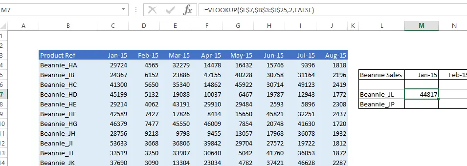
It can be really frustrating if you have set up your VLOOKUP formula, all is working great and then you have to manually adjust the formula if you want to copy it across multiple columns.
See my data below for an example of this scenario.

I want to look up the monthly Sales of of two types of Beannie hats in my total sales data. So, I have set up my VLOOKUP to look for monthly volumes of both Beanie hats Beannie_JL and Style Beannie_JP.

COLUMN translates a column number into a cell address. For example C1 would return 3 as C is the third column in our worksheet, so you can probably see how we can use this in the VLOOKUP formula.
=VLOOKUP($L$7,$B$3:$J$25,COLUMN(B1),FALSE)

Once I do this the formula will automatically updates as its dragged.
Want More VLOOKUP Tips?
 This post explored using a VLOOKUP formula combined with the COLUMNS Function. If you want more to answer any question using lookup formulas then I recommend Chandoo’s VLOOKUP Book. Click here to view more details