Hello, Excellers. Welcome to another #Exceltips #FormulaFriday blog post in my Excel 2021 series. The comparison of two Excel ranges for any differences is a common task. One way to do this to use conditional formatting to highlight differences between the two ranges.
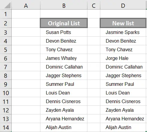
Take a look at my two lists below. I have an original list and a new list. Let’s go ahead and make the differences in these two lists stand out with conditional formatting.
First I want to create named ranges for each list. There are many benefits to using named ranges in your formulas.
- Formulas become more understandable or make more sense.
- Editing formulas become super easy.
- Creating formulas once ranges are set up become super fast.
Feel free to read my blog posts below for more details on names ranges.
Formula Friday – 3 Reasons To Use Named Ranges In Your Excel Formulas
Create A List Of Named Ranges In Excel. Excel Tip
Write A Macro Which Highlights Named Ranges. Macro Monday.
Macro Mondays – Create A Simple Excel Macro To Delete All Named Ranges.
Using Column And Row Labels As Named Ranges.
So, lets get back to our lists and naming the lists.
How To Create A Named Range.
There are a few ways to create a named range in Excel. Here are 3x ways as a lightning-fast guide on how to generate those names to help with conditional formatting.
Use the Name Box.
- Select the range of cell or cell you want to name.
- Click in the Name Box in the top left of the workbook.
- Name your cell or range of cells.
- Hit Enter.
Create Names From Worksheet Labels.
- Select the labels and the cells you want to name.
- On the Formula Ribbon – Defined Names – Create From Selection.
- Select the location of the label you want to use.
- Hit Ok
- Your selected name will appear in the Name Box.
Use The Name Manager.
- Formula Tab – Defined Names – Define Name
- Give your range a name
- Type in your value for this named range or use the selector to select a cell that contains your named data.
- Hit Ok
I have named the lists OldList and NewList. The original is the Old list and the new list is well New list. Makes sense right? This will make the conditional formatting formula easy to follow.
Step 1. Add Conditional Formatting To the Old List.
- Select cells in the OldList Range.
- Select Home | Conditional Formatting | New Rule.
- Once in the New Formatting Rule Dialog Box select Use a Formula to Determine Which Cells to Format.
- Enter the formula below in the dialogue box.
- =COUNTIF(NewList,B3)=0
- Click the Format button and the type of formatting you want to be applied if the condition in the formula is TRUE.
- I have chosen Orange.
- Hit ok.
Step 2. Add Conditional Formatting To the New List.
- Select cells in the NewList Range.
- Select Home | Conditional Formatting | New Rule.
- Once in the New Formatting Rule Dialog Box select Use a Formula to Determine Which Cells to Format.
- Enter the formula below in the dialogue box.
- =COUNTIF(OldList,B3)=0
- Click the Format button and the type of formatting you want to be applied if the condition in the formula is TRUE.
- I have chosen Green.
- Hit Ok.
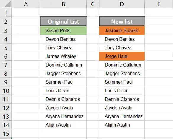
That’s all there is to it. Names in the Old List and not in the New List are highlighted, just as names in the New list but not in the Old List are too. Nice use of conditional formatting in Excel.
How Does This Work?.
The COUNTIF function counts the number of times a value appears in a range, If the formula returns 0 then it means the item does not appear in the range. The conditional formatting is applied in this case and the cell colour is changed.

