A really common task used frequently in Excel is to compare two lists to highlight items that appear in one list but are not in the other. Here is a great way to combine two great Excel features to get exactly the results we need.
We can combine the VLOOKUP function along with Conditional Formatting. The VLOOKUP will be used used to look up an item from one list in the other, and the Conditional formatting will highlight the missing items for us.
In my example I have two lists of products and suppliers and we want to check this list with the new list on the same sheet which has 3 products missing.
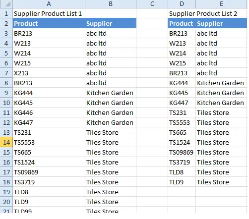
- Select the range of cells you wish to format, in my example it is A1:B21
- Hit Conditional Formatting on the Home Tab
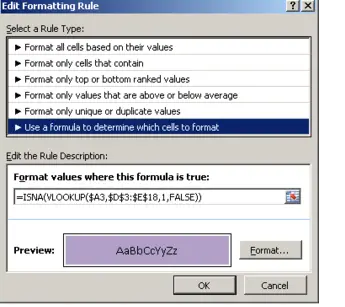
- Click Use A Formula To Determine Which Cells To Format
- Enter the VLOOKUP formula below into the field provided
=ISNA(VLOOKUP($A3,$D$3:$E$18,1,false))
So, the way this works is the Vlookup is looking for a match in column A. If no match is found the the error #N/A is returned. The ISNA function will return true if a match is not found, hence the cells will be formatted. Nice huh?
In my example I have found the three missing products of my second list stored in cell range D3:E18.

Want More VLOOKUP Tips?
