Hello Excellers and welcome to another #Excel #formulafriday blog post. Today let’s look at how to calculate average values in Excel based on a specific text string. We need to calculate the Quarterly Sales Values in this example. The specific string that we will be basing the calculation on is “North”, using an average formula in Excel.
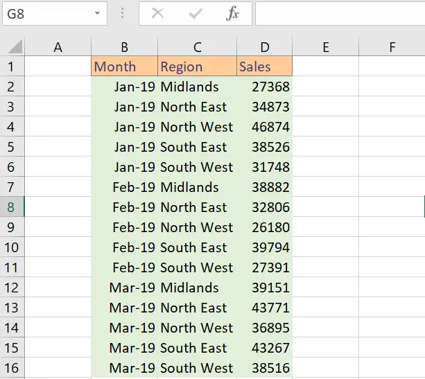
An extract of my Excel data set that I need to work with is in the screenshot below. I have the monthly sales values for a number of national sales regions. I need to quickly calculate the average quarterly sales for a specific region for the first quarter of the year.

To carry out this query we need to use an AVERAGE formula in Excel. In particular, it is the AVERAGEIF function which we make use of.
The AVERAGEIF Formula
So, let’s just jump back a little bit an explore the syntax of the AVERAGEIF Function in Excel. What does this formula do?. It is really straightforward.
It will return the arithmetic mean of a range of cells that meet a specific for given criteria.

Formula Syntax
AVERAGEIF(range, criteria, [average_range])
The AVERAGEIF function syntax has the following arguments:
Range. This is a required argument. One or more cells to average, including numbers or names, arrays, or references that contain numbers.
Criteria. This is also a required argument. The criteria will be in the form of expression, number, cell reference or text string. This is used to determine which cells are used to calculate the average value.”,
Average_range This is an optional argument. This refers to the actual set of cells to average. If this argument is omitted ( as it is optional), then the Range is used.
So, next we need to apply the function to our query. What are the average quarterly sales for any of our regions that contain the text “North”.
Writing Our Excel Formula Solution
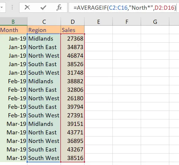
First, we start with the =AVERAGEIF instruction to Excel. This will prompt the formula dialogue box which takes us step by step through the arguments we need to enter.
- The first argument which is required is the Range.
In this example, it is the range C2:C16 .
- Second, we need to add our required criteria. We need to include all rows which relate to any region containing “North”. We are able to use a wildcard character in the criteria argument. The wildcard can be either a question mark (?). This matches any single character. Or we can use an asterisk (*), which matches any sequence of characters. Seeing as we need to search for any region with”North”, the asterisk seems to be the most appropriate.
- The final argument is the average range. This is an optional argument. We require this however, we need to calculate the average sales. We will use the cell range D2:D16 which contains our sales value data.

Extra Detail On The AVERAGEIF Function
- The Average_range and Range arguments do not need to be of the same shape or size of each other. The cells that are averaged are determined by using the top, left
cell in average_range as the beginning cell. Then, Excel includes cells that correspond in size and shape to the range. - Any cells that contain the values TRUE or FALSE are ignored by Excel.
- The #DIV/0! error value will be returned by the formula for a number of reasons
-No values match the specified criteria
-OR if the range is blank - If a cell in average_range is an empty cell, AVERAGEIF ignores it.
- If a cell in criteria is empty, AVERAGEIF treats it as a 0 value.
So, the answer to our question of the Quarterly sales of the total “North” region is

Have you used the AVERAGEIF function in Excel?. Share with us how you have used it and what problem it has solved for you.
If you want more tips then sign up to my monthly Newsletter where I share 3 Excel Tips on the first Wednesday of the month and receive my free Ebook, 30 Excel Tips.
Likewise, if you want to see all of the blog posts in the Formula Friday Series Click The Link Below
How To Excel At Excel – Formula Friday Blog Posts.
Other Related Blog Posts In The #Excel #FormulaFriday Series

