Hello, Excellers. It is Friday and that means some more #FormulaFriday Excel fun right?. If you need to number your table rows sequentially then this is the Excel tip for you.  So, if you sort your rows, or add new ones, the table always numbers the rows correctly sequentially rather than by just the number of the row that contains the formula.  We do this with the ROW function.

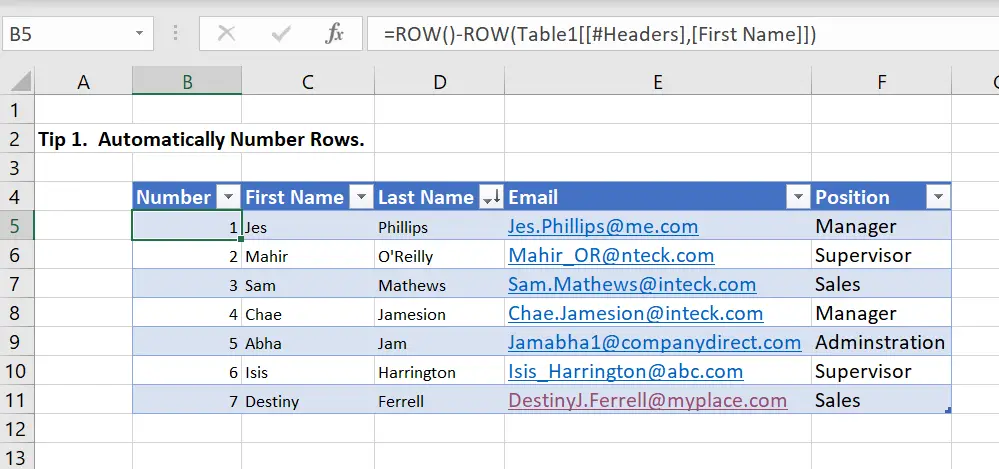
As always it is easier with an example to work with, see below. It a a small sample of dummy data which represents the structure of the original data set.

If you use the ROW function without any arguments, then it will simply return the number of the row.  It will not sequentially return the table rows.  So, create a calculated column using the formula below.

=ROW()-ROW(Table1[[#Headers],[First Name]])

So, how does this formula work?.   Here is the cool part.  If you use ROW with an argument as we have done here with a multi-row range then it will return the first row of the range. In this way, it will number the table rows.

In this example we are using column First Name column to indicate the the range.

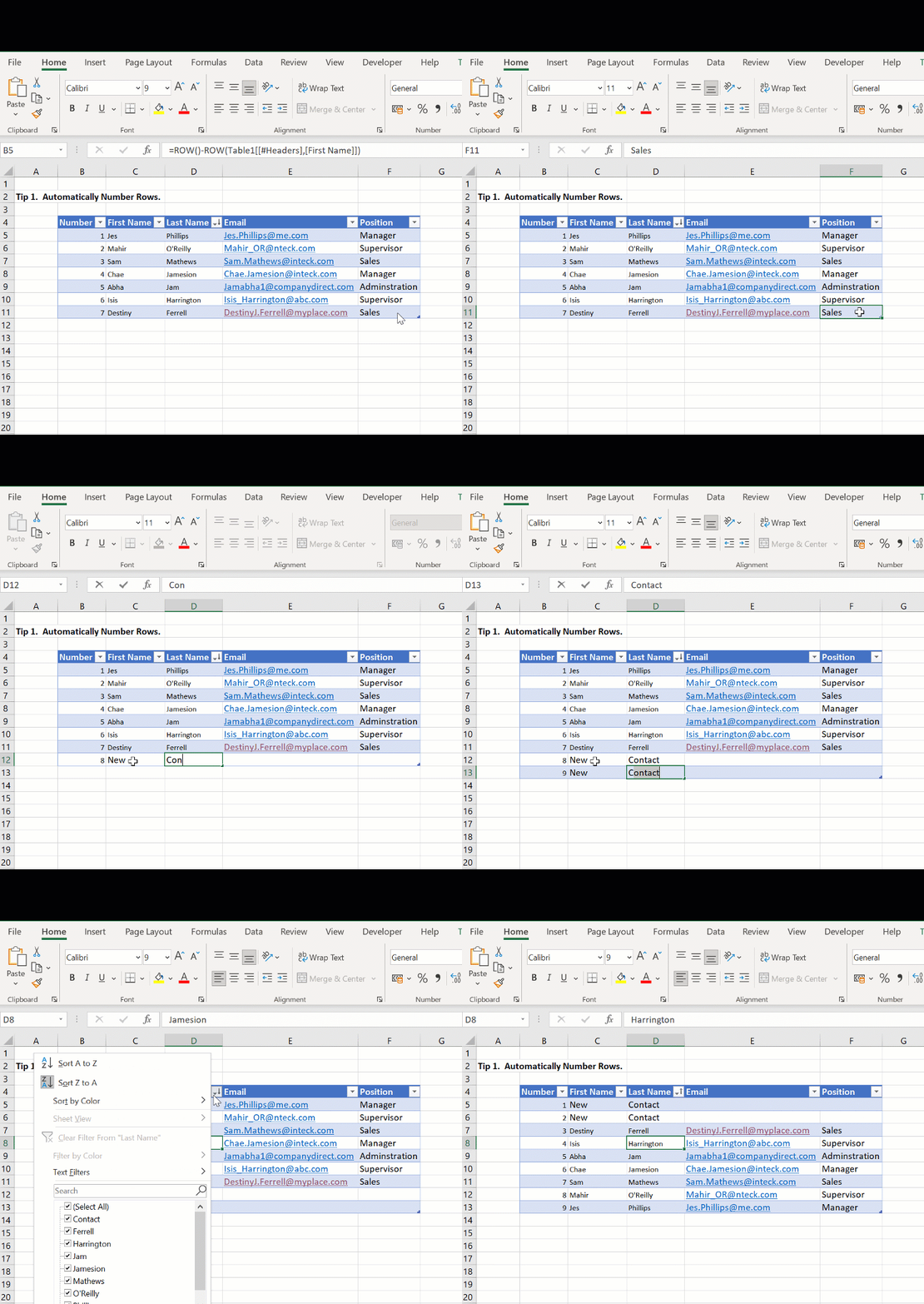
The numbers are now TABLE ROW number, not rows that correspond to the rows that contain the formulas. You can test this by sorting the table.  The number are sorted to TABLE ROW numbers. Will we test it?.

Great it works!  How cool is that?. Have you used the new Excel array function available with 365?.