Hello, Excellers. Welcome back to another #FormulaFriday #Excel blog post in my 2020 Excel series. Today’s blog will show you all you need to know about how to use Absolute (and Relative) references when you are using an Excel table and structured references.
Absolute Cell References.
I think one of the most useful and first thing we learn when using Excel is the value of using the $ symbol. (Or the F4) key. This allows you to freeze a column or row, so when dragging a formula down a column or across a row your cell reference does not change.
You can change a relative reference to an absolute one by the use of the $ as an addition to the formula. Here is a summary of where the $ should sit within your cell reference to achieve your constant or absolute cell reference.

The most commonly used absolute cell reference is that which anchors both the column and the row $A$1. All you need to do is hit F4 on your keyboard to make the cell reference absolute. You will find this is both the quickest and easiest way.
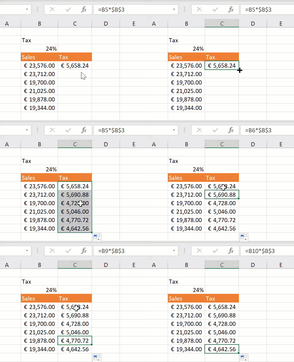
For example, if applying an increase of .05% increase in selling price to products, the increase can be referenced as an absolute cell reference. When the formula is applied or dragged down the list of products, the reference to the cell containing the sales increase does not move. See this in action below.
What About Structured References In Excel Tables?.
Once Excel Tables were introduced in Excel, cells were now referenced in a structured way. Here is a quick recap about structured Excel references.
Structured cell references are a special way to reference Excel tables. These type of references work the same as regular cell references but are a lot easier to understand and read. They also are dynamic and automatically adjust when data is added or deleted from an Excel table.
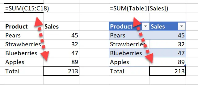
See the details of a quick example below. The SUM function with the usual range references, and on the right the Sum function with structured table references.
Structured Cell Reference Syntax.
Here is a very brief overview of the basics of the structured cell reference syntax to understand it better. Normally a structured cell reference begins with a Table reference (Table1 in our example above). This is followed by a column reference.
So, the reference has three parts.
- Table name
- Item specifier
- Column specifiers
Table Name. This is is the reference to the Table data without any row or column totals. If you have not named your table then this takes on the default name such as Table1 in our example.
Item Specifier. These are the specific parts of the table. You can see a summary in the table below of what can be used.

Column Specifiers. This references the data in the corresponding column. without the header row and total row. In the example we are using this could be [Sales].
So, back to using absolute references with tables. These structured cell references whilst have a number of benefits behave a bit differently. There is no way to create an absolute reference for a table reference within a formula. This is because, as by default all table references are absolute. When they are dragged or copied the following happens.
Column references change by referring to the next column to the right if you drag the formula across columns.
Column references do not change when copied or pasted, they remain static.
It is not as straightforward to anchor columns references as with a range reference to make them absolute. But there is a neat way to get around this.
So, when your formula contains a combination of absolute and relative references, there is no way to drag or copy the formula across and keep the references correct.
Here is the solution.
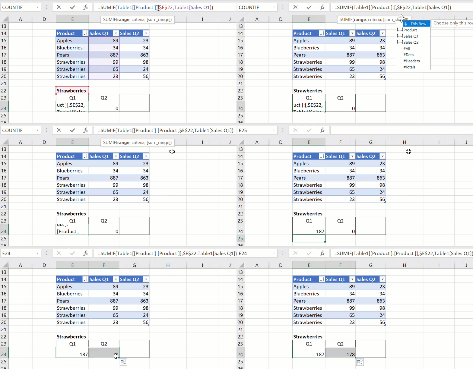
All we need to do is to add and additional and duplicate column reference. Duplicating the column reference anchors the reference when dragging across columns. Using the same example, I have added some extra data to work with. I have added Sales records for Q1 and Q2 and created a summary set to calculate sales of Strawberries for Q1. The formula is below.
=SUMIF(Table1[[Product ]],$E2$2,Table1[Sales Q1])
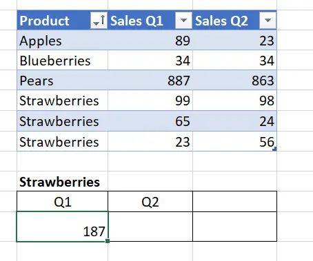
So, if I try to simply drag the formula across, as expected and already discussed above the formula does not move to calculate Q2 sales automatically. It moves the columns references to the right.
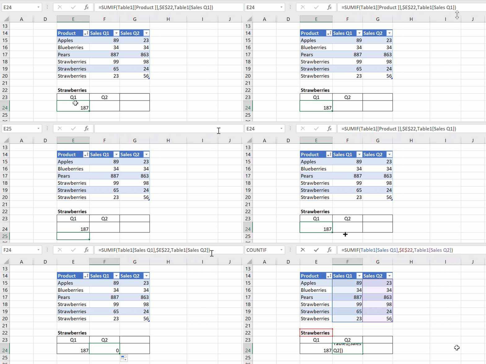
So, let’s add another additional and duplicate column reference to anchor the columns. This is the solution. I can now drag the formula across and get the right calculation.
