Hi Excellers, hope you are having an Excellent day. It is time for some more #formulafriday Excel formula fun. Today I have a Formula Friday Double edition. That’s right. Today I will show you how to create an ongoing count of sales orders we had in 2018. We will use two methods. Up to you which one you want to use. Both work equally well in Excel.
So, this tip is based on a question from a subscriber. They wanted to have an ongoing count of orders that are coming into the sales office on an ongoing basis throughout 2018.
The Example Data Set.
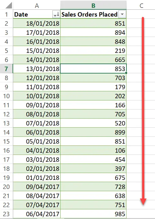
As ever let’s take an example dataset to work with both Excel formulas. Just as in the example question by my subscriber, the data set is an extract of daily sales orders placed. This is updated every morning. We want to automatically update the 2018 order volumes as they are updated from the sales order system. Our data set has records beginning in 2017.

So this is a double edition Formula Friday. That is right. We are going to explore TWO ways to get the same result. We are going to use the SUMIFS function in the first solution to this question of how to have an ongoing count of our orders.
SUMIFS Function – SOLUTION 1.
Let’s calculate how many sales orders came into our office to date in 2018. First, we can recap on the SUMIFS Function if you are new to it or have only used it once or twice. Its always good to start with the basic syntax.
SUMIFS is one of Excel’s Math and Trig Functions. It adds all of the values that meet multiple criteria. This sounds just the job for this query to have an ongoing count of orders.
=SUMIFS(sum_range, criteria_range1, criteria1, [criteria_range2, criteria2], …)
Where
sum_range – this is the range of cells you want to SUM.
criteria_range1 -(required) this is the range is being tested using criteria1
criteria1 – (required) the criteria that define which cells in criteria_range1 will be added.
Both criteria_range_1 and criteria1 are a pair where a search range is analysed for specific criteria. If those criteria are met then the corresponding values in the sum_range are added.
[criteria_range2, criteria2] – subsequent criteria argument are options pairs and up to 127 arguments can be used
Working Through Solution 1.
So, here is the solution to the problem to find the ongoing number of sales orders received in 2018 STEP BY STEP.
Step 1. Set the sum_range
=SUMIFS(Table1[Sales Orders Placed] in this example it is Column B (Sales Orders Placed).
Step 2. Set the criteria_range1
=SUMIFS(Table1[Sales Orders Placed],Table1[Date], in this example it is Column A (Date).
Step 3. Set the first criteria
=SUMIFS(Table1[Sales Orders Placed],Table1[Date],“>=01-Jan-2018” the first criteria is dates greater than or equal to 01-Jan-2018.
Step 4. Set the criteria_range2
=SUMIFS(Table1[Sales Orders Placed],Table1[Date],“>=01-Jan-2018”,Table1[Date], this is again Column A (Date)
Step 5. Set the second criteria
=SUMIFS(Table1[Sales Orders Placed],Table1[Date],“>=01-Jan-2018”,Table1[Date],“<=31-Dec-2018”) the first criteria is dates less than or equal to 31-Dec-2018.
This formula easily sums the number of sales order placed within 2018. As our data set is contained in an Excel Data Table, the formula is dynamic by nature and will automatically take into account new data lines as they are added to the dataset.
SUMPRODUCT Function – SOLUTION 2.
The second solution is using the SUMPRODUCT function. If you are new to SUMPRODUCT then let’s take a look at what exactly it does. In basic terms, it multiplies ranges or arrays together and sums the results. So first it multiplies, then it sums. It is a bit like using COUNTIF or SUMIF but with extra power. We can take a walk through the syntax first to see how this function can help solve this business problem as good as method 1.
=SUMPRODUCT (array1, [array2], …)
Where
array1 – The first array or range to multiply, then add.
array2 – [optional] The second array or range to multiply, then add. You can have up to 255 arrays within the formula.
So, here is the solution to the problem to find the ongoing number of sales orders received in 2018 STEP BY STEP.
Working Through Solution 2.
Step 1. Set array 1
=SUMPRODUCT(–(Table1[Date]>=DATE(2018,1,1))*–(Table1[Date]<=DATE(2018,1,31))
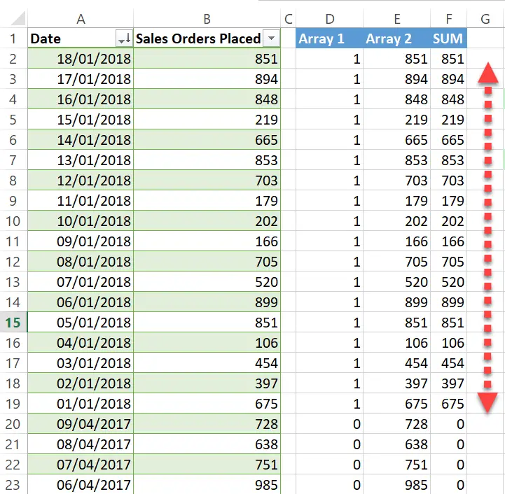
This first array is set as Column A (Date) and looks for the dates between 01 Jan 2018 and 31 Jan 2018. We can do this by incorporating the DATE function, if the condition is met then it is flagged as 1 if not then 0. By using the double negative — (double unary) we are able to coerce the TRUE/FALSE into the numeric values one and zero.
Step 2. Set array 2
=SUMPRODUCT(–(Table1[Date]>=DATE(2018,1,1))*–(Table1[Date]<=DATE(2018,1,31)),Table1[Sales Orders Placed])
Sales Orders Place are the second array in the this formula.
Excel multiplies all of the components of the two arrays, then sums or adds the products. You can see below what happens with our example formula. Where the dates are flagged as being within the date range with 1, the second array is then multiplied by this array and the product of these arrays summed or added. Clever stuff isn’t it.

To download the example data set and two solutions then you can click on the link below. Easily calculate your ongoing count of sales orders.
So, we have seen two methods to achieve the same results with two awesome Excel functions, SUMIFS and SUMPRODUCT. Let me know in the comments below which method you would use to solve this business problem. Are you a SUMIFS person or do you prefer to use SUMPRODUCT?.
Both methods work just as well, it’s just a matter of preference for me. I have used both to count ongoing sales orders.
Formula Friday Blog Posts.
If you want more Excel and VBA tips then sign up to my Monthly Newsletter where I share 3 Tips on the first Wednesday of the month and receive my free Ebook, 30 Excel Tips and check out all of my Formula Friday Blog posts below.
How To Excel At Excel – Formula Friday Blog Posts.
Do You Need Help With An Excel Problem?.
Finally, I am pleased to announce I have teamed up with Excel Rescue, where you can get help with Excel FAST. Why not check it out?.


