Recently a colleague was having an issue with their Pivot Table, they claimed some if their data was ‘missing’, a subscriber to my newsletter also had this issue so I thought I would cover it in today’s post.

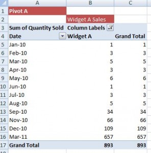
Let’s say if you have sales data for 12 months for 3 products, but unfortunately some months of the year those products did not sell any units (as in the data table shown below), you would still want to show the data for those products for those months even if none were sold. Check out the difference in the Pivot Tables below.

The months October 10 as well as january, February and April 11 have no A Widgets sold.

Pivot A shows data without zero values.

Pivot B shows the complete data set including those months and products with no units sold.

So, if your data looks a little strange or you think some is missing, then you may likely be unknowingly hiding zero values in your data.

My colleague breathed a sigh of relief, they thought that something had gone seriously worng with their data analysis.

So, if you are creating a pivot table which might offer this type of problem during creation, you can use the “Show Items with No Data” option to make sure that all of the months will appear. This is accessed in Excel 2007 via the following

1. Right clicking in the pivot table column area and selecting Field Settings- Layout and Print- Layout -Show Items with no data
2. Or click in your pivot table, Active Field- Field Settings- Layout and Print- Layout -Show Items with no data.

Other Excel Tips For You.

1. Quickly create a combination chart in Excel

2. The super quick one click chart

3. Create A self expanding chart in Excel

4. Is this THE simplest dynamic chart ever?