I have included this tutorial as part of the Pivot Table Tutorials as I have found to fully understand and get the best out of this fantastic Excel function you need to know the core terminology, concepts, functions and bulding blocks to getting your data set just right so you can have perfect pivots!

Let’s start with the basics. Pivot tables allow you to analyze a data set or this is sometimes referred to as a record set is simply a table or list of data which you could have typed into Excel yourself, or equally received as an output form an SQL query or an MS Access Database.

The Pivot Table will analyze the data in the data set, and will quickly allow you to summarize, perform calculations (without generating the formulas!!) on huge amounts of data all by dragging, dropping and selecting columns and rows and interactively moving them around to display the data summaries you want to.

Example

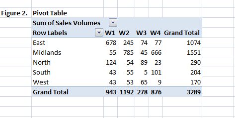
In the example below you can see the result of the raw data set in Figure 1, being summarized by a Pivot Table in Figure 2.

What’s With The Name?

So, why are they called Pivot Tables? Well, you literally can ‘pivot’ the data in different ways and immediately see it’s effect on your information as you move the data set around. If you take a look at the example below, we have a data set with sales people, area, product codes and volumes sold of the products.

In Figure 2 – the Pivot Table we can easily change the way the data is analyzed. Sales of product are being analyzed in the first instance by Sales Area, we can then easily add in the Sales person in a click or two.

But……Your Pivot Table is only ever as good as the data that you supply to it. We all know the saying Garbage In Garbage out , but more often that not its stronger than that….. S**T In S**T out as DATA is THAT important. So, here are a few guidelines for getting your data list or table in the correct format for your Pivot Table to feed on.

We talk about data tables earlier in this Tutorial. A data table is no more than a list which has more than one Column of data with a Heading for each of the columns. Its really important to get the structure of your data table or set correct as it is the basis for your Pivot Table. Once you know the concept of this, applying it is easy. Follow this best practice and you should have no issues with your Pivot Table data.

• Firstly, HEADINGS- these are essential for your columns. Each column should have its own unique heading. They should always be in the row directly above your data- no blank row between your columns heading and your data. Ensure that they stand out as heading- I ALWAYS bold my headings just so its obvious.

• Never have BLANK cells in your data. Repeat the data as many times as you need to but no blank cells.

• I usually leave three or four blank cells above my data set. I use these for formulas or additional information sometimes, but they can be hidden. Handy to have none the less

• If you have more than one data set and they are related then make them into one large table. Let Excel and Pivots do the hard work!. if they are unrelated but on the same sheet if you leave a couple of columns between them, then they will be reconised as seperate by Excel.

So, lets summarize.

You need a good data set or table, laid out in rows and columns, the columns must have unique headings. We do not want ANY blank cells, Pivots do not like them!

If you have more than one data set that is related combine them into one larger set of data and let excel do the work. If they are unrelated then have a column or two between the tables, Excel will recognize them as different sets of data.

Want to download a workbook to accompany this tutorial? Yo can do that right HERE.{filelink=7}