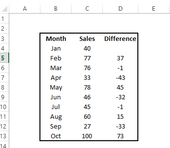
Most Excel users would be used to working with the concept of displaying negative numbers in a worksheet with a preceding – sign in front of the number, something a bit like this below, where I have an example of monthly sales and the diference month on month of those sales figures. The negative differences are easy to see.

So, how about making the positive numbers just as identifiable with a + sign in front of the numbers. It is really easy in Excel to create these formats using the custom number formatting feature in Excel.

There are varying monthly performances; the negatives are obvious so let’s go ahead and make the positive ones just as obvious.

Word of note….. If we apply only the positive formatting to the data range in the above example we will wipe the original formatting of the negative values, (not exactly what we want), we therefore need to also take into account negative values and ensure we re- apply formatting for them as well. This is just as easy to do at the same time as applying the postive conditional formatting.

• Select the range of cells you want to format.
• Home tab
• Number Group
• More number formats
• Custom

Or hit CTRL+1 to open the format cells dialog box

• Select Custom
• Type +0;-0;0
• Hit Ok

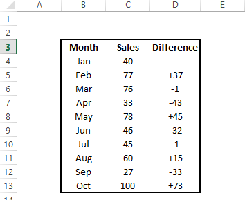
Here is the same set of data with the new formatting- what do you think?

Both the positive and the negative are appopriately formatted (+0;-0)along with the blank cell reference having no formatting at all. This is the last ;0 part of the formatting instructions to Excel.

Have you ever used this type of formatting?. Do you think it makes a difference to the the impact of the data at all?

How To Compress Picture Sizes In Excel

How To Change The Number Of Recently Used Files Excel Displays

How To Print An Entire Excel Workbook At Once

Control how many last used Files Excel displays for you

Prevent user printing an Excel workbook

Easily find your most often used Excel workbooks