When you need to sort and rank a field within a large number of data items it can be confusing to determine the ranking of the data you are looking at if the list is too long, or you may want to turn the Pivot Table into hard data for further analysis along with the ranking field.
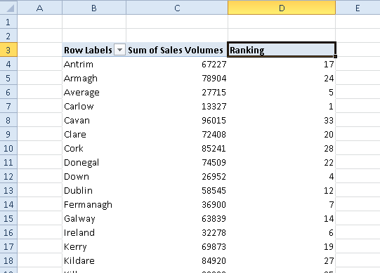
So, we can get Excel Pivot Table to show ranking which is really useful. Firstly create a Pivot Table as normal and add in your data measure twice as in my example below.
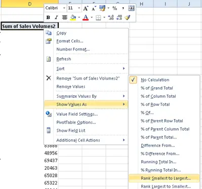
- Right click your second instance of your data measure
- Select Show Value As
- Rank Smallest To Largest
After the ranking has been applied, just adjust the labels and formatting to suit your taste and make your report look a bit better. There, easy ranking of your data fields in a Pivot Table.

Create Multiple Reports From One Pivot Table
Break Your Pivot Table Filters Into Multiple Columns


