If you create multiple charts in Excel, this tutorial is a game-changer. You may or may not have noticed that by default, Excel will create a Column Chart. You can easily set your preferred chart type as the default, streamlining your work effort and saving you valuable time. Who doesn’t want that right?.

Step 1. Create Or Select An Excel Chart.

First, to set up your default Excel chart type, you do not even have to create a chart at the same time. But if you have a chart already created, you can select it. If you do not, you can proceed by pressing the Alt+F1 key. This is the shortcut to make the default chart.

Step 2. Choose The Default Chart Type.

Right-click in the chart and select Change Chart Type. Alternatively, you can choose the Chart Design Tab and click Change Chart Type. Both give the same results.

 

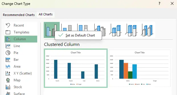
By selecting this option ( or the option you have selected for your most-used Excel charts), Excel will use this type of chart by default instead of the system default of Column Chart. How useful is that?

Of course, we need to test that Excel will create the new default I have chosen. Mine should default to a Clustered Column chart by default. Let’s give it a go. I hit F11 or Alt+F1. Yes, I get a Clustered Column chart.

 If you want more Excel Charting Tutorials, feel free to read my online Tutorials here.

If watching videos on your thing, then view my Excel Tutorial Videos here.