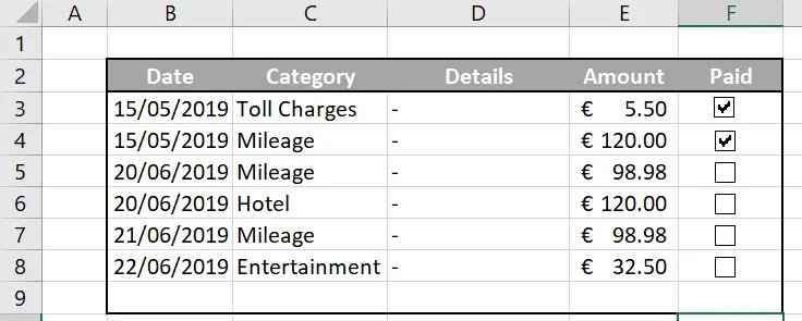
First of all, hello, Excellers. A warm welcome back today for another #Excel Tip in my #FormulaFriday series. I share today a neat way to use the conditional SUM function with a tick box in Excel. When you use the SUM function, Excel automatically includes all cells in the range that are not blank. To exclude specific cells from the sum, use tick boxes to select only the cells to be included in the calculation. Subsequently, this Excel tip derives from a question submitted by a subscriber. There is a need to sum only paid expenses on the worksheet. The paid expenses are identifiable by being ticked on the Excel worksheet. So, let’s write the solution to this question.
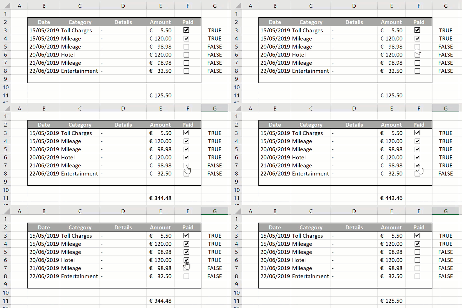
The cells being ticked or unticked determines the total amount paid in the solution.

The sample extract of the lists above demonstrates a list of expenses. A Check or Tick Box in Excel Column C will determine the status of the expenses. Ticked is paid, whereas unticked represents unpaid.
How The Excel Check or Tick Box Works In Excel.
The Check or Tick Box in Excel simply has a status of TRUE (ticked) or FALSE (un-ticked). This is pretty simple. So, once this is linked to a cell, a conditional SUMIF function is used to SUM the expenses. It is based on being TRUE is Paid or FALSE is Unpaid. The tick box is linked to cell C3. Below is how the TRUE or FALSE is displayed.

Adding A Check or Tick Box In Excel.
The Check or Tick Box control is available in the Developer Tab. Enable the Developer Tab if it is not visible. Follow the instructions below to enable the Developer tab.
- Click on the File tab of the ribbon to open the file menu.
- Select Options in the menu to open the Excel Options dialog box.
- Click on the Customize Ribbon option in the left hand window to view the available options in the right hand window of the dialog box.
- Under the Main Tabs section of the options window check off the Developer option.
- Click OK .
- The Developer tab is now visible
Now, insert the Check or Tick Box on the Excel Worksheet.
- Developer Tab
- Controls
- Insert | Form Controls
- Select CheckBox and place where you want to on your Excel Worksheet
Next, customize your CheckBox using the Format Control Option. Access this by right-clicking on the CheckBox. Select the cell link option, used with the conditional SUM or SUMIF Formula.
The link cell links to this expenses sheet are set up in Column G to the right of the CheckBox. So, if the Paid column cell is ticked the corresponding cell in Column G will display TRUE. Once unticked, Excel changes this value to FALSE.

So, TRUE and FALSE are then used to SUM the number of expenses. While only those flagged as TRUE will be used as the basis for the SUMIF function criteria. Let’s get writing that formula!.
Using The SUMIF Function. Basck To The Basics.
But, for now let’s get back to basics really quickly and look at the syntax of SUMIF. SUMIF is very straightforward but very powerful.
=SUMIF(range, criteria, sum_range)
Where
range – It is the data range you want Excel to evaluate.
criteria – Required. Enter the criteria in the form of a number, expression, a cell reference, text, or a function. This criteria defines the cells to sum. Note, any text criteria or criteria, including any mathematical or logical symbols MUST be enclosed in double quotation marks (“). For Example 31, “<31” ,A32, “Apples” etc.
Subsequently, the formula looks like below.
=SUMIF(G3:G9,”TRUE”,E3:E9)

So, the Check or Tick Box has changed the cell in Column C. Finally Excel adds the corresponding value to the total amount of Expenses Paid. How easy is that?. SUMIF is a flexible function and, combined with the Check or Tick Box in Excel, makes a solid solution in the example.
Have you used this method in an Excel template?. Share with other subscribers below. I would love to hear from you.
Feel free to take the sample Excel worksheet and play around with the sample data. Also I encourage you to read my selected and recommended blog posts below.
Finally, feel free to read all of the blog posts in the Formula Friday series click the link below.

