If you have been using Excel for a while you probably have used, or have been sent a spreadsheet with at least one hyperlink in them. These work really well until the order of sheets is changed, sheets are deleted or even new ones added. Then they don’t work as well and you will eventually get a warning that the link you want cannot be found. So, how about if you make your Excel Hyperlinks dynamic. Yes, that’s right, even if you move the sheets around, rename or add some more, your links will remain intact. Read on to find how to create dynamic hyperlinks using the hyperlink formula.

The Hyperlinks Function in Excel – Basics

Hyperlink Function Syntax

The syntax of the hyperlink function is=HYPERLINK(link_location, [friendly_name])

Where

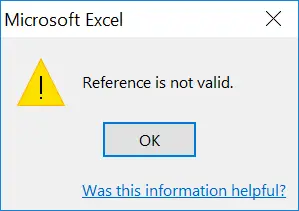
Link_Location – this is a required argument and is the file and path name to the document specified and can be another part of the same worksheet, workbook or opens up another workbook on the internet, intranet or a network server. If the link location cannot be found then an error will be displayed when you click on the hyperlink. It will look like the picture below.

If the friendly name argument returns an error, for example, #value then the cell will display the error. This will be instead of the jump text or value.

The Hyperlink Problem

Just as I stated at the start of this blog post if you change the name of worksheets, move them around or even delete some then you probably will run into problems with your hyperlinks.

The Dynamic Hyperlink Solution

I did also say at the top of this blog post there is a solution. Yes, let’s make our Excel hyperlinks dynamic. It is a simple process.

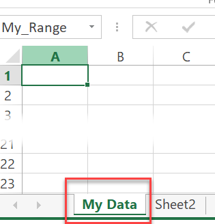
Select a cell in the worksheet that you want to link to. In this example, it will be Sheet 1 cell A1.  Enter a name for this cell. I am calling it MyRange.